Data Processing

The module analyzes vector and raster data online/offline. In addition, it supports data registration and projection transformation.

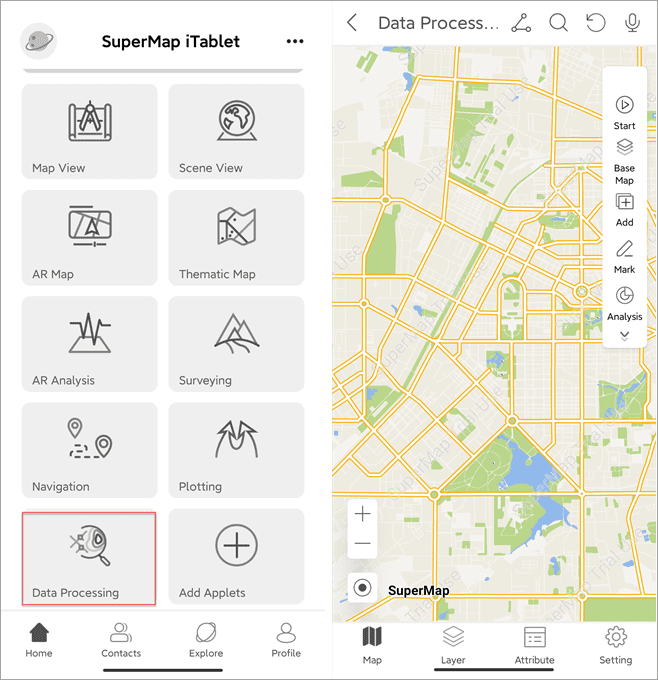
On the Home page click Data Processing to access the module.

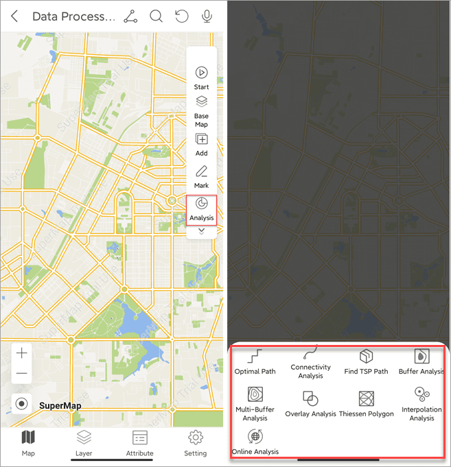
Data analysis

• Click the Analysis button and select an analyst.

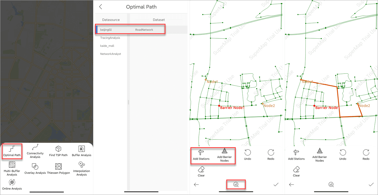
Optimal Path

• Click the tool Optimal path. Then specify your datasource and dataset.
• Click Add Stations and Add Barrier Nodes (optional) and press on the screen to add stations and barrier nodes. Click the Analyze icon on the center of bottom toolbar to get the result.

Buffer analysis

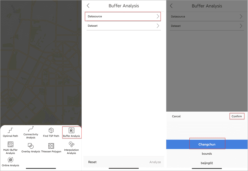
• Click Buffer Analysis and specify your datasource and dataset.
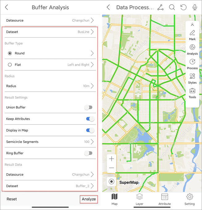
• After setting all buffer parameters click the Analyze button on the right bottom to get the result.

• Parameter description

Datasource: it is the datasource where your dataset for the analysis is located.

Dataset: the dataset for the analysis.

Buffer Type: the required parameters vary from the data types. When generating buffers for line data, either the round or the flat type can be chosen; when creating buffers for point or region data, only the round type can be chosen. A flat buffer can be unsymmetrical, with its right radius and left radius unequal, or with only one side.

Round: Two parallel lines are drawn at a certain distance of a line object, one on each side. A half-circle, with the buffer distance as its radius, is drawn to connect the same-side ends of the two parallel lines to form a buffer. Round is the default buffer type.

Flat: When generating a buffer, a rectangular buffer is formed by taking the line segment connecting adjacent nodes of a line object as one side and the left or right radius as the other.

Left: Create buffers on the left side of lines.

Right: Create buffers on the right side of lines.

Radius: the radius of buffer. It must be numerical.

Result Settings:

Union Buffer: If this option is checked, a Union operation will be performed on the generated buffers resulting in one complex buffer. If it is unchecked, generated buffers will remain unchanged in the result and no union

Keep Attributes: If this option is checked, the corresponding buffers will reserve the non-system field information of the original object. Otherwise, the non-system field information will be lost.

Display in Map: If this option is checked, the generated buffers will be added in the current map window. Otherwise, the buffer analysis result will not be added in the window.

Semicircle Segments (1-100): This parameter is used to set the smoothness of the buffer boundaries in the result. The greater this value is, the more circle segments there will be, and the smoother the buffer boundaries will be.

Result Data:

Datasource: Select the datasource for saving the resulted buffers.

Dataset: Input the name of the dataset where the generated buffers will be saved.

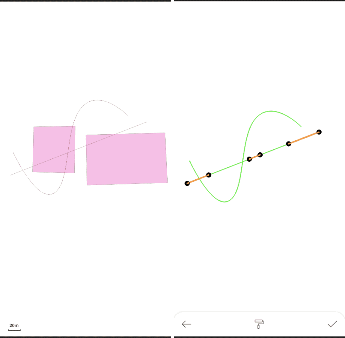
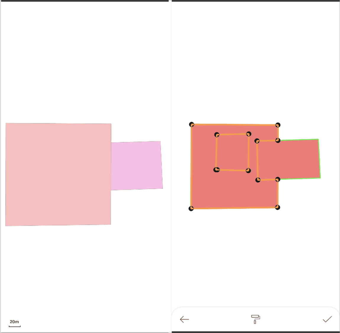
Overlay analysis

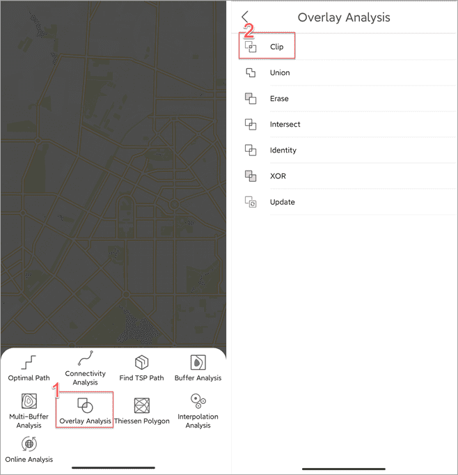
• Click Overlay Analysis and select an overlay type.

• Click Datasource, specify the source datasource and dataset, and click Confirm. Use the same way to set overlay data and result data. After all settings, click Analyze on the right-bottom corner.

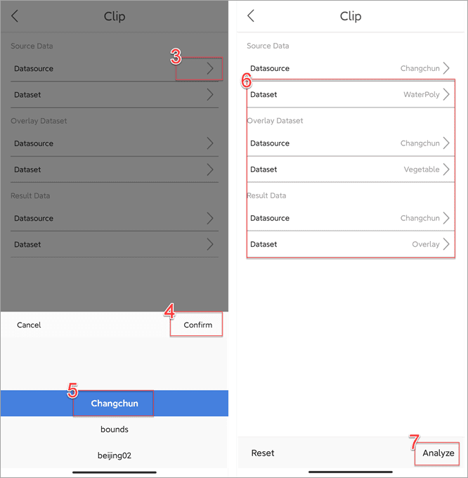
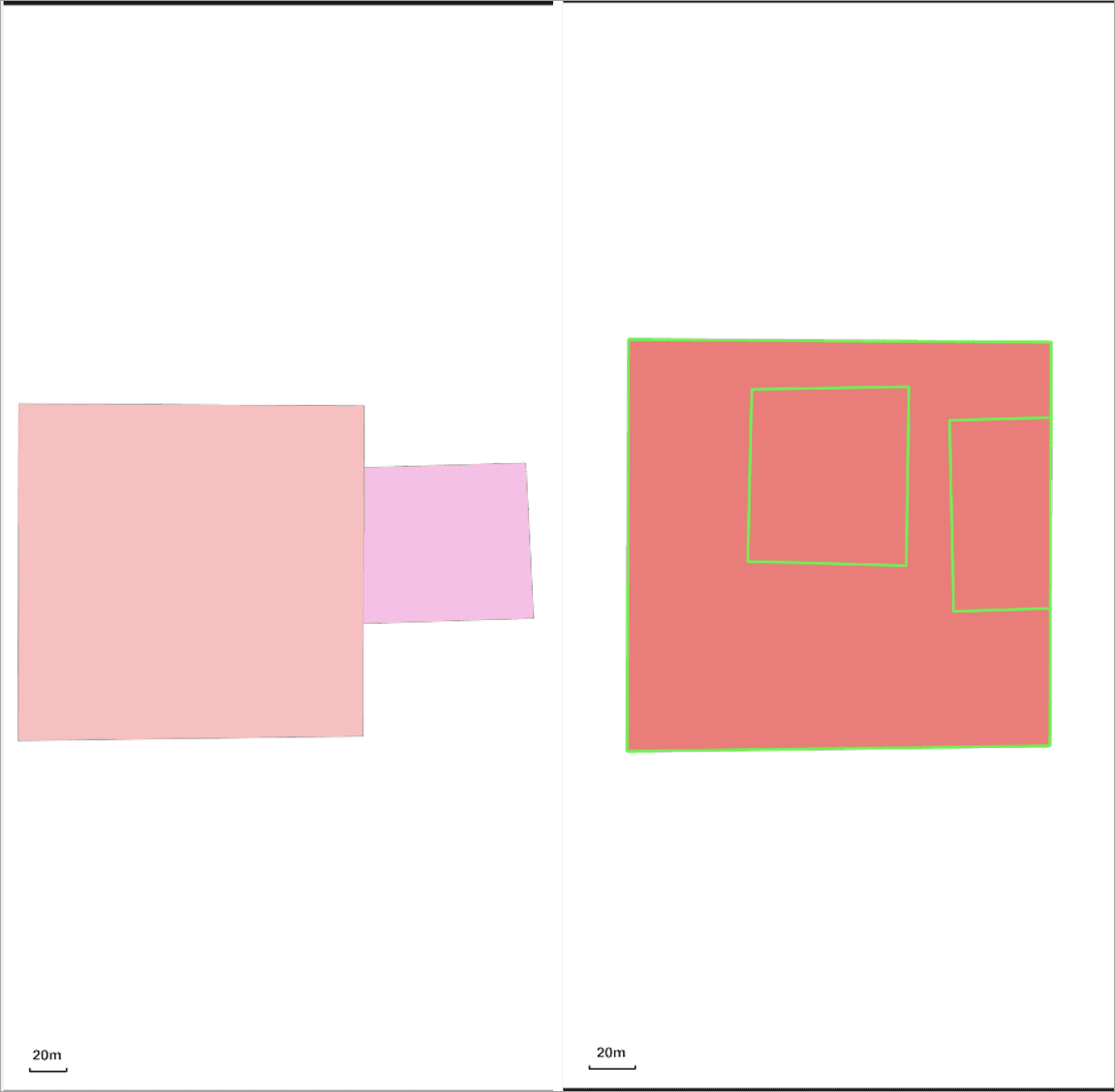
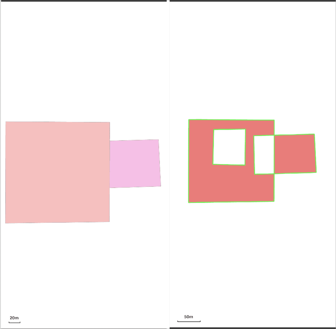
iTablet provides multiple overlay methods, including Clip, Union, Erase, Intersect, Identity, XOR, and Update.

• Clip: The clip dataset (overlay dataset) must be a region dataset, while the clipped dataset (source dataset) can be a point, line, or region dataset. Only the clip objects falling within the clipped polygons will be output to the result dataset.
• Merge: performs a Union operation on a source dataset and an overlay dataset.
• Erase: The erase dataset (overlay dataset) must be a region dataset, while the erased dataset (source dataset) can be a point, line, or region dataset. Only the erase objects falling outside of the erased polygons will be output to the result dataset.
• Intersect: The intersect dataset (overlay dataset) must be a region dataset, while the intersected dataset (source dataset) can be a point, line, or region dataset. The overlapped parts of the two datasets are reserved in the result dataset.
• Identity:

For the point dataset: the resulting dataset will keep all objects of source dataset.

For the line dataset: the resulting dataset will keep all objects of source dataset, but the lines that intersect with objects of overlay dataset will be split at each intersection.

For the region dataset: all the source datasets polygons that lie within the controlling boundary will be retained in the result dataset, and the objects are split at each intersection with the overlay dataset.

• XOR: The symmetry difference analysis on two region datasets. For each region object, the operation erases the overlapped part between the two datasets from the source dataset and reserves the rest part.

• Update: erases the content that overlays with the overlay dataset from the source dataset, and then paste the corresponding data of the overlay dataset to the source dataset. The result dataset keeps the geometric shapes and attribute information of the overlap dataset.

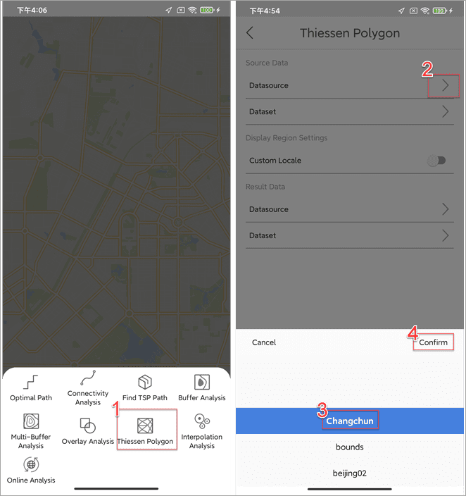
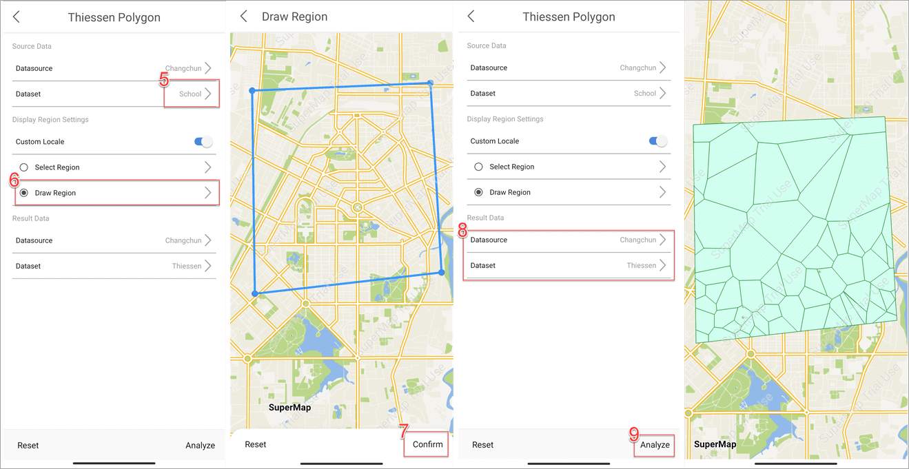
Thiessen polygon

• Click Thiessen Polygon, set source data and result data, and click Analyze. The default range of Thiessen polygons is the same as the source dataset. You can enable the Custom Locale parameter, and then specify a region object or draw a polygon as the range of Thiessen polygons.

Select Region: if your map exists the visible region layer, you can select one region object as the range of the resulting Thiessen polygons.

Draw Region: You can draw a region object as the range of the resulting Thiessen polygons.

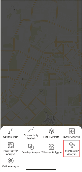
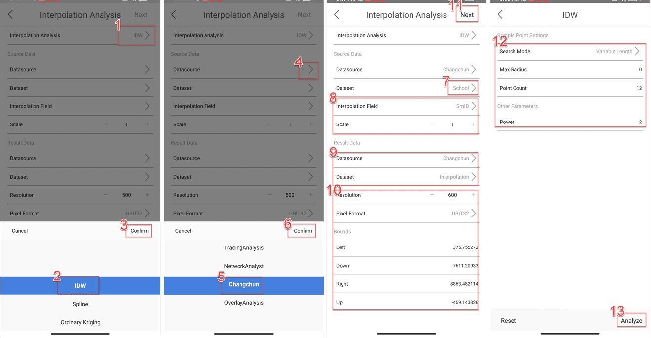
Interpolation analysis

• Click Interpolation Analysis to open the Interpolation Analysis page, and then choose a method from the Interpolation Analysis list.
• Specify the source data and the resulting data, set the analysis parameters, and click the Next button on the right-top corner. After setting all parameters, click the Analyze button on the right-bottom corner.

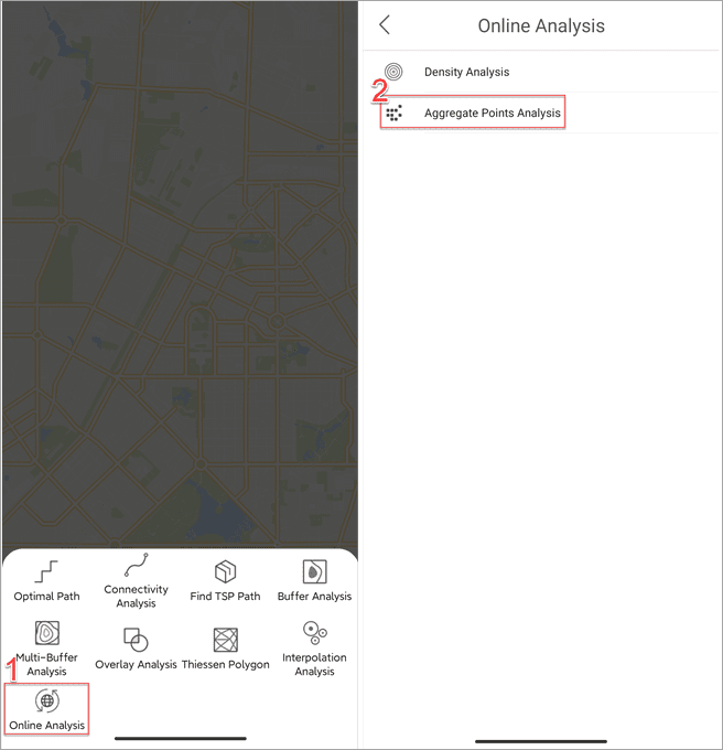
Online analysis

• Note: before an analysis, please deploy distributed analysis services on SuperMap iServer first.
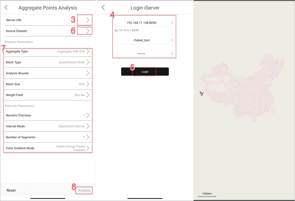
• Click Online Analysis and select an analysis type.

• Click iServer URL and enter service address, username, and password to log in to SuperMap iServer.
• Specify the source data, set parameters, and click the Analyze button on the right-bottom corner.

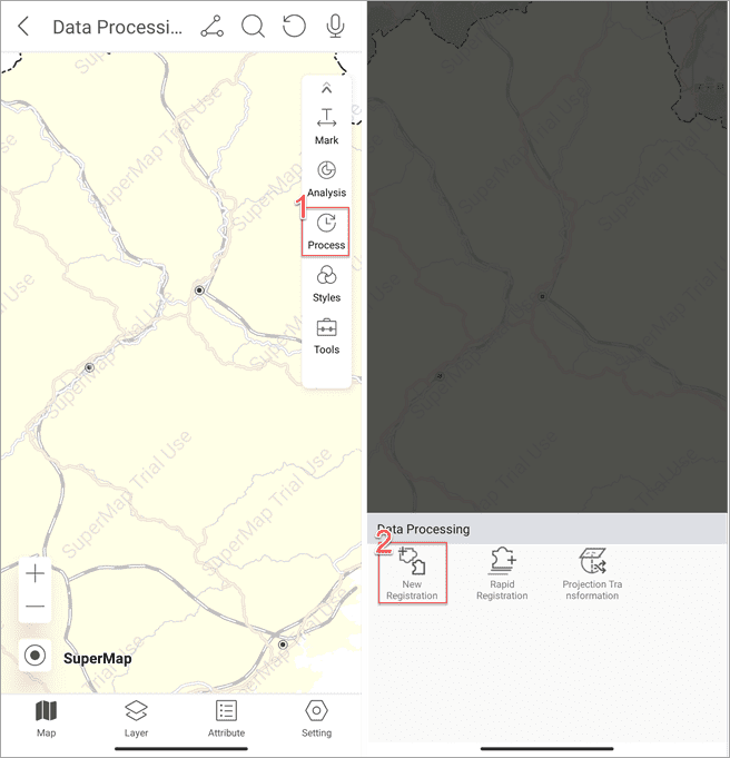
Data processing

New registration

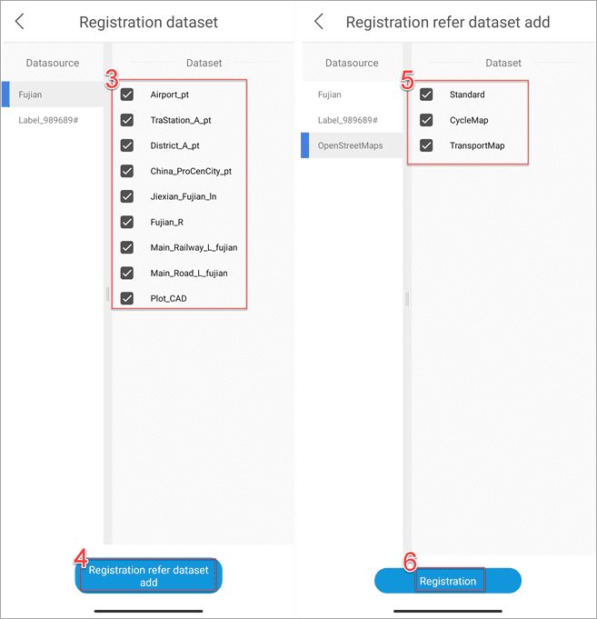
• After accessing the Data Processing, click the Process button on the right toolbar and select New Registration.

• In the Registration dataset page specify registration data and reference data. click Registration.

• Click Association to zoom the registration data and reference data synchronously. And then click Cancel the association to zoom data separately.
• Click Arithmetic on the right toolbar and select a method.

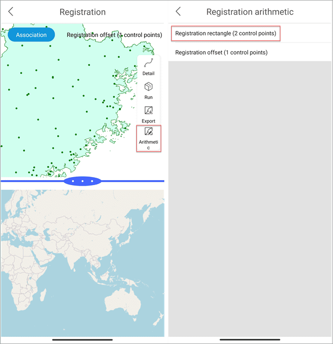
• Add two control points separately on the registration data and reference data.
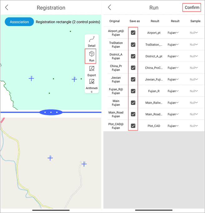
• Click Run to perform the registration. In the Run page you can check Save as to save as the resulting dataset. After all settings, click Confirm to finish the operation.

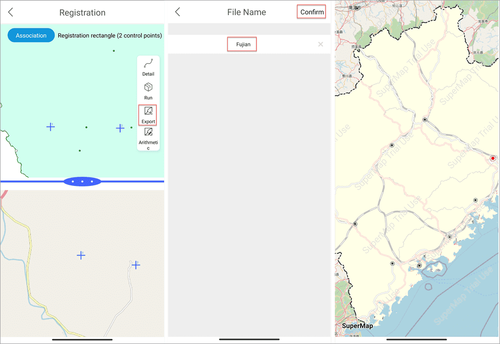
• After the registration, you can click Export on the right toolbar to export the registration information for further use.

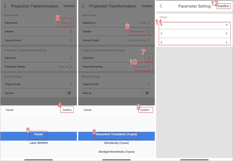
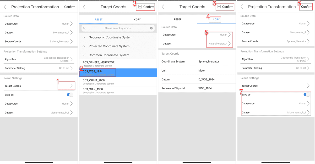
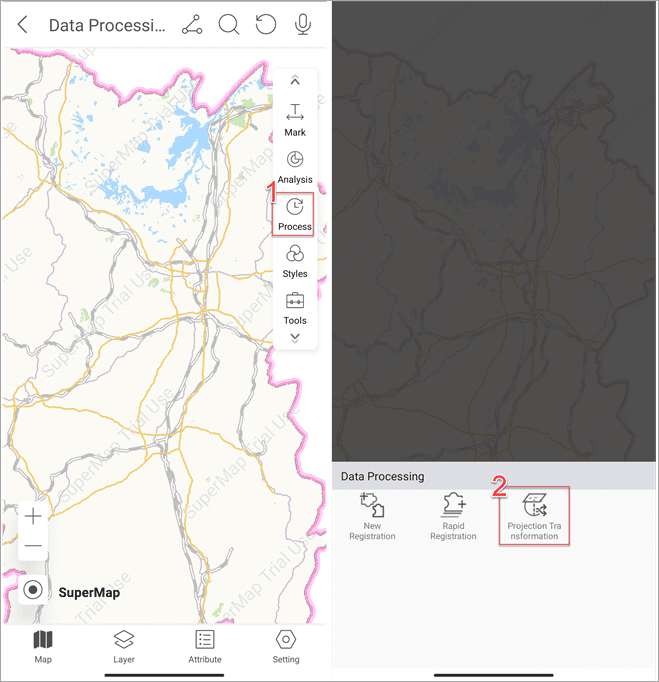
Projection transformation

• Note: the feature can be performed on data using geographical coordinate systems or projected coordinate systems.
• After accessing the Data Processing, click Process > Projection Transformation.

• Set the source data, select the transformation algorithm, and specify the target coordinate system. You could specify a dataset to use its coordinate system as the target.
• Enable Save as to save as the resulting dataset.
• After all settings, click Confirm.