Spatial Autocorrelation

Feature Description

Measures spatial autocorrelation based on feature locations and attribute values using the Global Moran's I statistic. Evaluates whether the pattern expressed is clustered, dispersed, or random.

Analysis Principle

The statistical value of spatial autocorrelation can be calculated using the following formula:

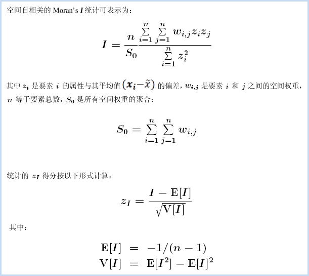
The mathematical formula underlying the Global Moran's I statistic is shown above. This tool calculates the mean and variance of the evaluated attribute. Each feature value is then subtracted from the mean to obtain deviations. The product of deviations for all adjacent features (e.g., those within a specified distance range) is summed to form the numerator of the Global Moran's I statistic.

After calculating the index value, the Spatial Autocorrelation (Global Moran's I) tool computes the expected index value. The observed index value is then compared to the expected value. Based on the number of features and data variance, the tool calculates z-score and p-value to determine statistical significance. The index value should be interpreted in the context of the null hypothesis.

Application Scenarios

Determine appropriate neighborhood distances for spatial analysis methods by identifying peak distance (where spatial autocorrelation is strongest)
Measure overall trends of racial/ethnic segregation over time - is segregation increasing or decreasing?
Summarize spatial-temporal spread of opinions, diseases, or trends - do they remain concentrated or become dispersed?

Feature Entry

Spatial Statistics Tab -> Analyzing Patterns -> Spatial Autocorrelation
Toolbox -> Spatial Statistics -> Analyzing Patterns -> Spatial Autocorrelation

Parameter Description

Source Dataset: Specifies the vector dataset for analysis (point/line/polygon). Recommended minimum 30 features for reliable results.
Analysis Field: Numeric field containing attribute values for analysis.
Conceptualization Model: Defines spatial relationships between features:
- Fixed Distance: Suitable for point data or polygon data with varying sizes
- Polygon Adjacent (Common Edges/Intersect): For adjacent polygons sharing edges/intersections
- Polygon Adjacent (Node/Common Edges/Intersect): For polygons sharing nodes/edges/intersections
- Inverse Distance: All features influence each other with weights inversely proportional to distance
- Inverse Distance Squared: Similar to Inverse Distance with faster distance decay
- K Nearest Neighbors: Considers K nearest features with equal weights (1), excludes others (0)
- Spatial Weight Matrix: Uses spatial weight matrix file (.swmb) reflecting distances/time/costs between features
- Undifferentiated Region: Combines fixed distance and inverse distance models
Distance Threshold: "-1" computes default distance (ensures minimum 1 neighbor); "0" considers all features as neighbors; positive values define adjacency range
Inverse Distance Power: Controls distance decay rate (higher values = faster decay)
Number of Neighbors: Positive integer specifying K nearest neighbors (required for K Nearest Neighbors model)
Distance Measurement: Euclidean Distance or Manhattan Distance (see Spatial Statistics Glossary)
Spatial Weights Matrix Standardization: Recommended for skewed distributions. Normalizes weights (0-1 range) by dividing each weight by row sums. Particularly useful for administrative boundaries.

Result Interpretation

Analysis results are stored in CAD Dataset and displayed on the map.

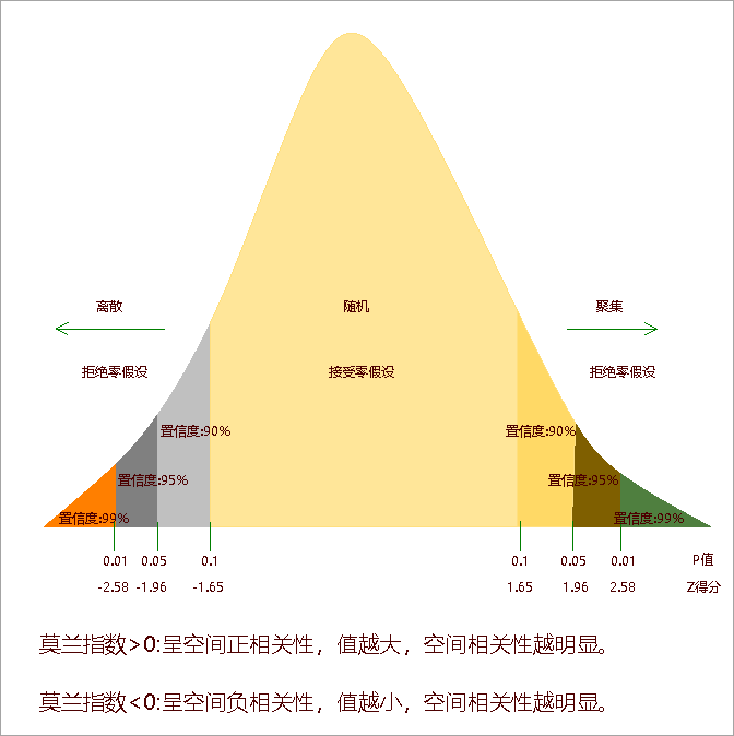
Results include: Moran's I Index, Expected Value, Variance, Z-score, and P-value. A significant z-score/p-value indicates rejection of null hypothesis. Positive Moran's I suggests clustering, negative value indicates dispersion:

Example

Sample Data: Download case data (requires extraction after download)

Using viral hepatitis incidence data from a province, spatial autocorrelation analysis was performed with:

Analysis Field: Case count
Conceptualization Model: Inverse Distance
Distance Measurement: Euclidean Distance
Spatial Weights Matrix Standardization applied

Results show:

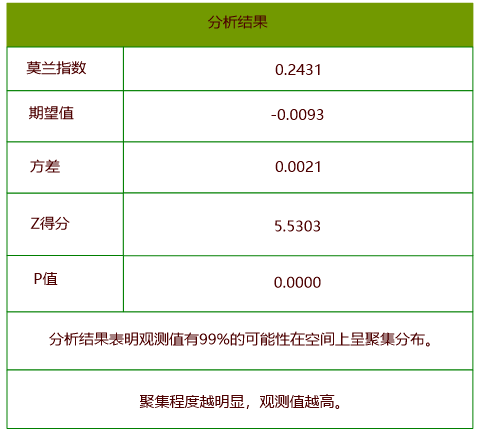
Conclusion: With p-value < 0.01 and z-score > 2.58, the analysis shows 99% confidence in significant spatial clustering (Moran’s I > 0).