Basic Vocabulary of Spatial Statistics

The theoretical foundation of spatial statistics is based on statistics. Understanding basic statistical terms and concepts will facilitate the comprehension of spatial statistics functionalities.

Null Hypothesis

A statistical term referring to the default assumption established prior to hypothesis testing. When the null hypothesis holds true, relevant statistics should follow specific probability distributions. If computed statistics fall into the rejection zone, it indicates a low-probability event has occurred, leading to rejection of the null hypothesis. In spatial statistics, the null hypothesis assumes spatial randomness - either spatial data follows random distribution, or values associated with spatial data exhibit random spatial distribution. As shown in the figure below, if your calculation result falls within the -2 to 2 range, your hypothesis is acceptable; otherwise, it indicates a low-probability event.

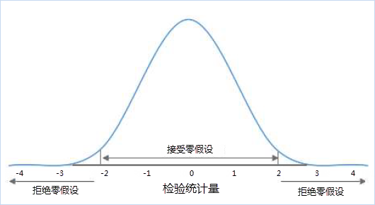
Example: If N criminal incidents occurred in a city during February with no additional conditions, they should theoretically be evenly distributed across all areas - this constitutes the "null hypothesis". In spatial statistics, the null hypothesis implies completely random (uniform) spatial distribution within a given region. Actual crime distribution might show clusters (some areas with multiple incidents and others with none). We determine whether to accept or reject the null hypothesis through analysis of P-value and Z-score.

P-value

The P-value represents probability, indicating the likelihood of observed events. In spatial statistics, it denotes the probability that observed spatial patterns occur randomly. When the P-value is sufficiently small, it suggests the observed spatial pattern is unlikely to result from random processes, justifying rejection of the null hypothesis.

Z-score

The Z-score measures standard deviation multiples, reflecting dataset dispersion. Both Z-scores and P-values relate to standard normal distribution. Critical values are illustrated below:

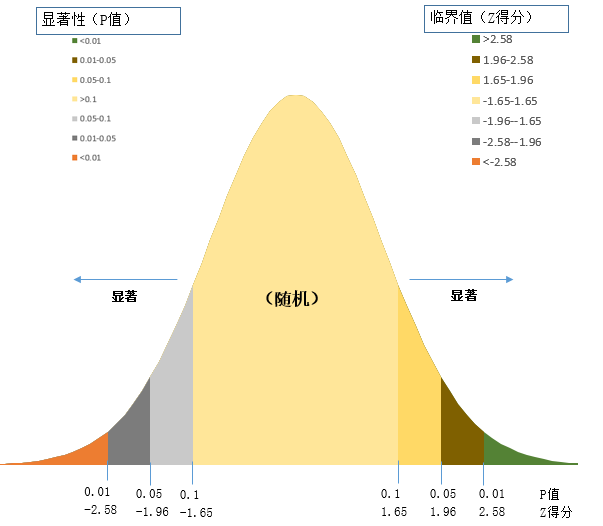
As shown, P-values and Z-scores typically appear together. Extremely high/low Z-scores (negative values) at the tails of normal distribution correspond to very small P-values. When analysis yields small P-values with extreme Z-scores, this indicates observed spatial patterns significantly deviate from theoretical random patterns under the null hypothesis, suggesting clustered or dispersed data distribution.

Confidence Level

Spatial statistics employs inferential statistics by establishing a null hypothesis assuming random spatial patterns of features or associated values. The P-value determines the probability of accepting/rejecting the null hypothesis, while the Z-score indicates standard deviation multiples for identifying clustering/dispersion.

Typical confidence levels are 90%, 95%, or 99%. For example, when P < 0.1, there's 10% probability of randomness and 90% probability of clustering/dispersion, justifying null hypothesis rejection.

The table below shows uncorrected critical P-values and Z-scores at different confidence levels (FDR correction may apply):

Z-score (Standard Deviation)	P-value (Probability)	Confidence Level
<-1.65 or>1.65	*<0.10	90%
<-1.96 or>1.96	*<0.05	95%
<-2.58 or>2.58	*<0.01	99%

Morans

Moran's I is a crucial spatial autocorrelation measurement. As a normalized rational number ranging from -1.0 to 1.0: Moran's I >0 indicates positive spatial correlation (stronger values denote more pronounced clustering); Moran's I <0 shows negative spatial correlation (lower values suggest greater dispersion); Moran's I = 0 implies spatial randomness.

Centroid

While spatial statistics accepts point/line/polygon datasets as input, spatial relationships like inverse distance require actual spatial distance calculations. For measurement purposes, centroids are used: weighted mean centers for all sub-features. Weighting factors are 1 for points (self-coordinates), length for lines, and area for polygons.

Self Weight

Certain spatial statistics functions allow users to specify a numeric field representing self-weights (distance/weight between a feature and itself). Typically zero, user-defined values in the weight field will override default settings in calculations.

Distance

Spatial statistics employs two distance metrics: Euclidean and Manhattan.

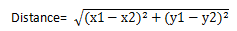
Euclidean distance measures straight-line distance between Cartesian coordinates (x1,y1) and (x2,y2):

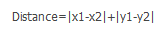
Manhattan distance calculates axial projection sums between points:

Regression Analysis

Regression analysis identifies quantitative relationships between variables. Categorized as linear/nonlinear based on variable relationships. Simple linear regression involves one independent and one dependent variable with linear correlation. Multiple linear regression extends to two or more independent variables.

Spatial Weight Matrix

A spatial weight matrix quantifies spatial relationships between dataset features (N×N table where N=feature count). Each cell value represents spatial relationship weight between row and column features. Conceptualization should match actual interactions (e.g., inverse distance for seed dispersal analysis vs travel time for commuter distribution).