


Measures spatial autocorrelation for a series of distances. Z-scores reflect the intensity of spatial clustering, and statistically significant peak z-scores indicate distances where spatial processes promoting clustering are most pronounced. Peak distances are typically used as parameter values for functions with "distance range" or "distance radius". When performing analyses like hot spot analysis (Getis-Ord Gi*) or density analysis, selecting an appropriate distance is crucial. You can first use incremental spatial autocorrelation to determine a suitable distance.
Feature Entry
- Spatial Statistics Tab -> Analyzing Patterns -> Incremental Spatial Autocorrelation.
- Toolbox->Spatial Statistics->Analyzing Patterns->Incremental Spatial Autocorrelation.
Parameter Description
- Source Dataset: Specifies the vector dataset for analysis, supporting point, line, and polygon datasets.
- Evaluation Field: Sets the property field values of features participating in the analysis. This field should contain varied values; if all objects have the same value (e.g., 1), the calculation will fail. Only numeric fields are supported.
- Starting Distance: The initial distance for incremental spatial autocorrelation analysis, which can be determined based on data clustering patterns. If unspecified, the default value is the minimum distance where each feature has at least one neighbor. This default may not be optimal if spatial outliers exist in the dataset.
- Incremental Distance: The interval distance between consecutive analyses. Subsequent analyses use the starting distance plus this incremental value. If unspecified, the smaller value between the average nearest neighbor distance and (Md - B)/C (where Md is the maximum threshold distance, B is the starting distance, and C is the number of distance bands) will be used. This ensures calculations adhere to the specified number of distance bands and prevents excessive maximum distances where features might consider nearly all others as neighbors.
- Number of Distance Bands: Specifies the total analysis iterations for the dataset, ranging from 2 to 30.
- Distance Measurement Method: Supports Euclidean distance and Manhattan distance. For detailed descriptions, see Spatial Statistics Basic Vocabulary.
- Spatial Weights Matrix Standardization: Recommended when feature distributions might be biased due to sampling design or aggregation schemes. Standardization divides each weight by the sum of row weights (sum of weights for all neighboring features). This is typically used with fixed-distance neighbors or polygon adjacency relationships to mitigate bias from varying neighbor counts. It scales weights between 0 and 1, creating a relative weighting scheme. Always select this option when working with administrative boundary polygons.
Result Description
Analysis results are presented as tabular data and visualized in a statistical chart window. The table includes six fields: incremental distance, Moran's I, expected value, variance, Z-score, and p-value. Z-scores indicate spatial clustering intensity, with statistically significant peaks identifying distances where clustering processes are strongest. These peak distances are often optimal values for parameters like "distance range" or "distance radius".
Example
Using microblog login data from a city to study hotspot patterns and spatial aggregation, with login counts as the evaluation field. Before performing hot spot analysis (Getis-Ord Gi*) or kernel density analysis, incremental spatial autocorrelation determines an appropriate distance parameter. Sample results are shown below:
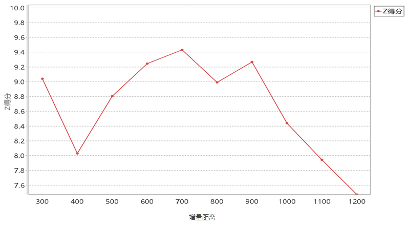
As illustrated, when the incremental distance reaches 700 meters, the Z-score peaks, indicating 700 meters is the optimal radius for hotspot analysis of microblog login data.
Related Topics