High/Low Clustering

Feature Description

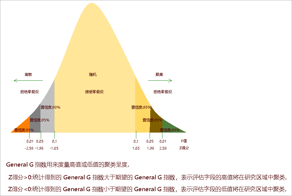
High/Low Clustering measures the degree of clustering for either high values or low values using the Getis-Ord General G statistic. The General G Index is an inferential statistic that uses limited data to estimate characteristics of the entire population. When the returned P-value is small and statistically significant, we can reject the null hypothesis. In such cases, a positive Z-score indicates the observed General G Index is larger than expected, suggesting clustering of high attribute values in the study area; a negative Z-score indicates the observed General G Index is smaller than expected, suggesting clustering of low attribute values.

Application Cases

Detecting abnormal peaks in emergency room visits may indicate outbreaks of local or regional health issues.
Comparing spatial patterns of different retail industries in urban areas to understand competitive sectors (e.g., car dealerships) and non-competitive sectors (e.g., health centers/gyms) through comparative shopping analysis.
Assessing the degree of spatial clustering over time to examine changes, such as analyzing urban population clustering patterns during urban development and densification processes.

Feature Entry

Spatial Statistics Tab -> Analyzing Patterns -> High/Low Clustering.
Toolbox -> Spatial Statistics -> Analyzing Patterns -> High/Low Clustering.

Parameter Description

Source Dataset: The vector dataset to analyze, supporting point, line, and polygon datasets.
Evaluation Field: The numeric field representing attribute values for analysis.
Conceptualization Model: Defines spatial relationships between features. More realistic models yield more accurate results.
- Fixed Distance: Suitable for point data and polygon data with varying sizes.
- Polygon Adjacent (Common Edges/Intersect): For polygons sharing edges or intersections.
- Polygon Adjacent (Node/Common Edges/Intersect): For polygons sharing nodes, edges, or intersections.
- Inverse Distance: All features influence each other with weights inversely proportional to distance, suitable for continuous data.
- Inverse Distance Square: Similar to inverse distance but with faster distance decay (weights = 1/distance²).
- K Nearest Neighbors: Uses K nearest features with equal weights (1). Effective for ensuring minimum neighbors and handling uneven distributions.
- Spatial Weight Matrix: Uses a spatial weight matrix file (.swmb) to model spatial relationships, ideal for network-based analyses like crime cluster detection.
- Undifferentiated Region: Combines fixed distance and inverse distance models. Features within a threshold have equal weights; others follow inverse distance rules.
Distance Threshold: "-1" calculates default distance; "0" treats all as neighbors; positive values define adjacency range.
Inverse Distance Power: Controls distance decay rate. Higher values reduce distant influences faster.
Number of Neighbors: Specifies K for K Nearest Neighbors model.
Distance Measurement: Euclidean Distance or Manhattan Distance. Details in Spatial Statistics Glossary.
Spatial Weights Matrix Standardization: Normalizes weights by row sums (0-1 range), recommended for administrative boundaries to reduce bias from varying neighbor counts.

Result Interpretation

Analysis results are stored in a CAD dataset and displayed on the map.

The High/Low Clustering analysis returns five parameters: General G Index, Expected Value, Variance, Z-score, and P-value. As an inferential statistic, a small P-value (<0.05) allows rejecting the null hypothesis. A positive Z-score indicates high-value clustering; a negative Z-score indicates low-value clustering:

Use High/Low Clustering to detect spatial peaks of high values in uniformly distributed data. When high and low clusters cancel out (observed G ≈ expected G), consider Spatial Autocorrelation analysis instead.

Example

Sample Data: Download case data (requires extraction after download).

Analyzing viral hepatitis incidence using: Evaluation Field = case count, Conceptualization Model = inverse distance, Distance Measurement = Euclidean, Standardized spatial weights. Results show:

Conclusions: P-value <0.01 and Z-score >2.58 indicate 99% confidence in significant high-value clustering of hepatitis cases.