


The grid Surface Analysis function of SuperMap is a Based on the surface modle and obtain information or generate surface., mainly including:
Isolines are  extracted
Contours are one of the common ways to represent a surface on a map. An isoline is a smooth curve connecting adjacent points of equal value. Commonly used contour lines are: contour, isobath, isotherm, isobar, isohyet, and so on.
The distribution of contours reflects the variation of values on the surface of the grid. The denser the distribution of contours, the greater the variation of values on the surface of the grid. For example, in the case of contours, the denser the distribution of contours, the steeper the slope. In the case of contours, the sparser the distribution of contours, the smaller the variation of values on the surface of the grid. In the case of contours, the slope is very gentle. By extracting the isoline, we can find the position where the values of elevation, temperature and precipitation are the same, and the distribution of the isoline can also show the steep and gentle areas of change.
Key Concepts
- Base value and equidistance
- Smoothness and Smoothing Methods
The reference value is the initial starting value when the isoline (surface) is generated. It is calculated in the forward or backward direction with the isoline distance as the interval. Therefore, the reference value is not necessarily the value of the minimum isoline (surface). The reference value may be any number.
The contour distance is the interval value between two adjacent contours, which together with the reference value determines which contours are extracted.
The value and the number of the extracted isolines can be determined by the two parameters. For example, if the base value is set to 0 and the contour distance is set to 50, for a DEM Raster Data with an elevation value in the range of 120-999, the minimum extracted contour line is 150, the maximum extracted contour line is 950, and a total of 17 contour lines can be extracted.
The contour line is generated by interpolating the original Raster Data and connecting the contour points, so the result is a broken line with sharp edges and corners. Smooth Line is needed to simulate the real contour line. The user can perform Smooth Line on the generated contours by using different smoothing methods and setting different Smoothness.
Smoothness is in the range 0, 5. A value of 0 or 1 indicates that Smooth Line is not performed. The higher the value of Smoothness, the higher the smoothness. A Smoothness setting of 3 is generally recommended.
SuperMap provides two Smooth Line methods, the B-spline method and the angle grinding method. Both of these methods make the extracted contours smoother with the increase of Smoothness. Of course, the larger the Smoothness is, the more time and memory are required for the calculation.
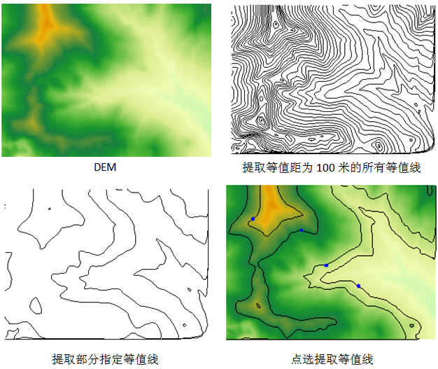
SuperMap supports Surface Analysis from the Raster Dataset to extract contours. Surface Analysis provides three isoline extraction methods: Extract All Isolines, Extract Specific Isolines and Isolines from Click.
- Extract All Isolines You can specify all qualified isolines in the Extract Surface model by specifying the parameter. Two parameters, reference value and contour distance, are generally used to control the extracted contour.
- Extract Specific Isolines You can specify a certain number of isolines of specific values as required by the user. You can enter values for the isolines directly, or you can automatically generate a series of level values based on the range and interval you set.
- Isolines from Click Select isoline interactively by user clicking on the grid surface model. The result will output the isoline whose value is equal to the elevation of the selected point. Note that not only the isoline where the point is located.
 |
| Figure: Sketch of the extracted contours |
Extract Isosurface
An isosurface is a surface consisting of adjacent isoline closures. The change of the isosurface can directly show the change between adjacent isolines, such as elevation, temperature, precipitation, pollution or atmospheric pressure, which is very intuitive and effective. The effect of isosurface distribution is the same as that of isoline distribution, which also reflects the change on the grid surface. The denser the isosurface distribution, the greater the change on the grid surface value, and vice versa, the less the change on the grid surface value. The narrower the isosurface, the greater the change on the grid surface value, and vice versa, the less the change on the grid surface value.
SuperMap Surface Analysis provides two methods to extract isoregions: Extract All Isoregions and Specified Isoregions.
- Extract All Isoregions All qualified isosurfaces in the Extract Surface model can be specified by the parameter. Generally, two parameters, reference value and isosurface distance, are used to control the extracted isosurface. The reference value is used as an initial starting value for generating an isosurface; the isodistance is an interval value between two isolines, and the number of the extracted isosurfaces can be determined by the two parameters. For example, if the base value is set to 0 and the iso-distance is set to 50, for the DEM Raster Data with the elevation value in the range of 120-999, the minimum iso-surface value extracted from all iso-surfaces is 150, the maximum iso-surface value is 950, and a total of 16 iso-surfaces can be extracted. The iso-surface is generated by interpolating the original Raster Data, connecting the iso-points to obtain the iso-line, and then closing the adjacent iso-lines, so the result is a polygonal surface with clear edges and corners, and a certain Smooth Line is needed to simulate the real iso-surface. The smoothing method for the iso-surface is the same as that for the iso-line. SuperMap also supports two smoothing methods: the B-spline method and the angle grinding method.
- Specified Isoregions You can specify a certain number of specific values as required by the user. You can enter a specific value directly, or you can automatically generate a series of level values based on the range and interval you set.
 |
| Figure: Extract Isosurface diagram |
Line-of-sight Analysis
Line-of-sight Analysis, also known as line of sight analysis, essentially belongs to the category of terrain optimization. Line-of-sight Analysis has important application value in navigation, aviation and military affairs, such as setting up radar stations, transmitting stations of TV stations, road selection, navigation, etc. In military affairs, such as setting up positions, setting up observation posts, laying communication lines, etc; Sometimes it is possible to analyze the invisible area. For example, when a low-altitude reconnaissance aircraft is flying, it is necessary to avoid the capture of enemy radar as much as possible, and the aircraft should choose the radar blind area to fly. There are two basic contents of Line-of-sight Analysis: one is Visibility Analysis between two or more points; the other is Viewshed Analysis, that is, for a given observation point, analyze the area covered by the observation.
The viewport is the range of the earth's surface that can be seen from one or more observations. Viewshed Analysis is to find the intervisibility coverage area of a given observation point within a given range based on a certain relative height on Raster Dataset, that is, the intervisibility area range of the given point. Analyst Result is a Raster Dataset. Viewshed Analysis is used to determine the location of transmission towers, the area scanned by radar, and the establishment of forest fire watchtowers.
When performing Viewshed Analysis, you need to specify several important parameters, including observation point, Append:, View Radius:, View Angle:, and so on.
- Observation point: The observation point is the origin for Viewshed Analysis, which can be one or more. When there are multiple viewpoints, it can be determined that some viewpoints can see a common viewable area.
- Append:: The height of the observation point consists of two parts, one is the surface elevation of the observation point, and the other is Append:. Therefore, the height of the observation point can be adjusted by the Append: of the observation point. For example, if the actual ground elevation of the observation point selected on the map is 430 meters and the Append: value is 100 meters, the elevation of the observation point is 530 meters.
- View Radius:: View Radius: limits the scope of the viewfield search. If you want to find the visible range of the observation point only within a certain length, you can specify the visible radius, and the visible range is found within a circular range with the observation point as the center and the visible radius as the radius. The default value of the view radius is 0, which means View Radius: infinity, that is, looking within the entire Map Bounds.
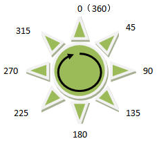
- View Angle:: View Angle: restricts the search direction of the viewfield. View Angle: In degrees, between 0 and 360 degrees. The default Start Angle is 0 degrees, starting from due north and rotating clockwise to 360 degrees.
SuperMap supports Viewshed Analysis for a single point as well as for multiple observation points. Observation points can be added either by mouse click or by Import Dataset. It also supports the Export as Point dataset, which will be selected in the map.
Multi-point Viewshed Analysis
Multi-point Viewshed Analysis is to find all the areas that can be viewed by all the observation points within the given range based on the relative heights of the given observation points on the Raster Data surface, and the Analyst Result will get a Raster Dataset. The multi-viewshed can be a Common viewshed (the intersection of all viewsheds) or a non-Common viewshed (the union of all viewsheds).
In multi-point Viewshed Analysis, it is also possible to have a separate Append: value for one or more observation points. When the elevation is attached, it is likely that the result obtained by assigning Append: is quite different from that obtained by not considering Append:. Therefore, it is very important to know the height of the observation point and add Append:.
Multi-point Viewshed Analysis can form multiple observation points by directly clicking multiple points on the grid map; it can also generate multiple observation points by Import Point Dataset. The imported Point Dataset can have Elevation Field or unified Set Appended Altitude value.
The Analyst Result of the viewfield of multiple observation points is shown in the following figure:
 |
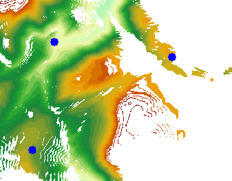 |
| DEM Dataset and Observation Points | Multi-point Viewshed Analysis result |
Visibility Analysis Based on the given observation point and target point, the input grid surface is analyzed to see whether they are visible or not. According to the number of observation points, the SuperMap Surface Analysis provides 2-Point Visibility Analysis and multi-Point Visibility Analysis respectively.
- Two-Point Visibility is used to analyze whether any two points on the earth surface can see each other.
Because the digital elevation model describes the elevation of ground points and does not include the height of objects on the ground, such as forest trees and buildings, when the height of objects has a non-negligible impact on the Analyst Result, you can add the "Append: value" to adjust the height of the observation point to get the correct result. If Append: is entered, the elevation is appended to both points, and it is likely that the result obtained by appending Append: is diametrically opposite to that obtained by not considering Append:. For example, if Append: is not considered, the two points are invisible, and if Append: is considered, the latter two points are visible. So knowing the figure height and adding Append: is important in some cases. 2-The Point Visibility Analysis can directly draw two points on the grid map for analysis, and can also analyze the intervisibility of point objects in the imported Point Dataset.
- Multi-Point Visibility is used to analyze whether multiple points on the grid surface can see each other.
In the Multi-Point Visibility Analysis, we can append: values to one or more points individually. After the elevation is attached, it is likely that the result obtained by appending Append: is diametrically opposite to that obtained by not considering Append:. So knowing the figure height and adding Append: is very important in some cases.
Multi-Point Visibility Analysis can be directly selected on the grid map of the mouse to form a number of points involved in the analysis of the point; can also be generated through the Import Point Dataset of the way involved in the analysis of the point.

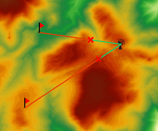
DEM Dataset and Observation Point Multi-Point Visibility Analysis Result The 3D Spatial Analysis function is the sublimation of the 2D Spatial Analysis function, which is intuitive and vivid. As shown in the figure below, it is the presentation effect of Multi-Point Visibility Analysis in the scene.
Multi-Point Visibility Analysis effect in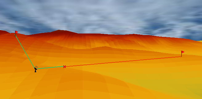
3D Scene
Slope and aspect
Slope and aspect are two important factors of terrain characteristics, which play an important role in terrain Surface Analysis. Where slope is a measure of the rate of change of altitude at a point on the surface of the earth, and the direction of change of slope is the aspect, which is a measure of the change of direction of the slope at a point on the surface of the earth.
When you want to build a house on a mountain, you need to find a relatively flat area on the mountain; if you want to build a ski resort on the mountain, you need to choose different slopes to be used as a primary slide, an intermediate slide and an advanced slide to meet different levels of ski enthusiasts; when a rescue plane involved in an emergency lands, you need to find a relatively flat area on the ground. In addition, in the grade of cultivated land slope, it is stipulated that 25 ° is the limit slope for reclamation, and it is not allowed to plant in wasteland above 25 °. For these problems, the slope of the terrain needs to be considered.
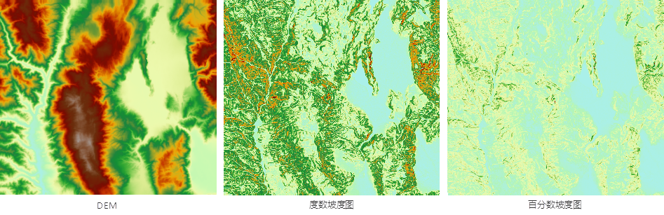
The slope of a point on the surface of the earth is a quantity that represents the degree of inclination of the earth's surface at that point, and is a vector with both magnitude and direction. In terrain analysis, slope represents the angle between a tangent plane passing through a point on the surface of the earth and the horizontal plane. According to the slope map, the steepness of the terrain at each location in the area can be understood. In the slope map, each pixel has a slope value, the larger the value is, the steeper the terrain is, and the smaller the value is, the flatter the terrain is.
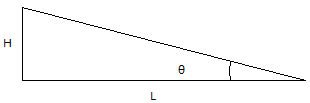
The slope may be expressed in degrees or in percent, where the degree slope is the arctan of the ratio of the vertical increment to the horizontal increment, and the percent slope is the ratio of the vertical increment to the horizontal increment multiplied by 100. In SuperMap, the slope calculation provides three representations: degrees, radians, and percentages. If the vertical increment of the slope is H and the horizontal increment is L, the angle is θ = arctan (H/L), the radian is R = θ * π/180, and the percentage is P = (H/L) * 100, as shown in the following figure.
 |
The Analyst Result for degree slope ranges from 0 to 90 °, where 0 indicates a horizontal surface and 90 ° indicates a steep surface perpendicular to the horizontal surface. The Analyst Result of percentage slope ranges from 0 to infinity. When the result is less than 1, it means that the elevation increment of the slope is less than horizontal increment, and the slope is gentle. When the result is equal to 1, it means that the elevation increment of the slope is equal to the horizontal increment, and the slope value is 45 °; When the result is greater than 1, it means that the elevation increment of the slope is greater than horizontal increment, and the slope becomes steeper.
The pixel value of Raster Dataset (GRID) is the value of the center point. When calculating the slope and aspect, the elevation value of each point can be obtained by interpolation, and then the slope and aspect of each point can be calculated. Since it is meaningless to calculate the slope and aspect of a point, this method calculates the average slope of each pixel plane in Raster Dataset.
 |
Slope aspect is of great significance in the fields of Vegetation Analysis and environmental assessment. There is generally a marked difference in biology between vegetation growing on slopes facing north and those growing on slopes facing south. The main reason for this difference is the difference in the adequacy of sunlight for the growth of green vegetation. When siting wind power plants, consideration should be given to building them on slopes facing the wind; Geologists often need to understand the major slope aspects of faults, or fold outcrops, to analyze the process of geological change; in determining the location of residential areas vulnerable to snow melt water, they need to identify south-facing slopes to get the location of the original melted snow.
The aspect of a point on the surface of the ground indicates the orientation of the slope passing through that point. In terrain analysis, the slope direction refers to the angle between the projection of the normal line of the tangent plane passing through a point on the earth's surface on the horizontal plane and the direction of due north passing through the point. Aspect indicates the direction of maximum change in the elevation value at that point.
Aspect is expressed in degrees, and the Calculate Aspect Result can range from 0 to 360 degrees. Start at 0 ° due north, move clockwise, and end at 360 ° due north. The value of each pixel in the slope map represents the direction of the slope of its pixel surface. A flat slope has no direction and is assigned a value of -1.
 |
Since aspect is a measure of roundness, 10 ° aspect is closer to 360 ° than 30 ° aspect. Therefore, before using the slope aspect for data analysis, the user needs to convert the slope aspect, that is, divide the slope aspect into four basic directions of east, west, south and north (or eight basic directions of east, west, south, north, southeast, southwest, northeast and northwest), and the conversion can be completed through the Raster Reclassifying function to highlight the range of the slope aspect to be considered.
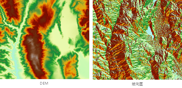 |
Table Surface Cut Fill
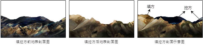
The migration of surface materials is often caused by sedimentation and erosion, which is manifested by the increase of surface materials in some areas and the decrease of surface materials in some areas. In engineering, it is common to refer to a reduction in surface material as "cut" and an increase in surface material as "fill." The area and size of fill/cut required to change one situation to another. The following figure shows the topographic profile of fill and excavation.
 |
Two Raster Datasets are required for grid mass haul calculation: Raster Dataset for Before Cut Fill and Raster Dataset for After Cut Fill. Each pixel value of the generated Result Dataset is the change value of the corresponding pixel value of the two Input Data sets. If the pixel value is positive, the surface material at the pixel is reduced; if the pixel value is negative, the surface material at the pixel is increased. As shown in the following figure, the Calculator Method of mass haul is displayed as a 4 * 4 Raster Data:
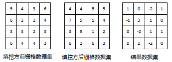 |
This figure shows that Result Dataset = Before Cut FillRaster Dataset-After Cut FillRaster Dataset.
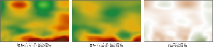
The following figure shows the Cut Fill Result diagram, which lists the Source Dataset before the mass haul, the Cut and Fill Data set as a reference, and the resulting mass haul Result Dataset. In the Source Dataset and Cut and Fill Data sets, higher elevation values bias the grid color toward brown-red; lower elevation values bias the grid color toward green. In the Mass Haul Result Dataset, the part that needs to be excavated is represented by dark green, and the greater the amount of excavation, the darker the color; the part that needs to be filled is represented by brown, and the greater the amount of filling, the darker the color; the part that does not need to be filled is represented by white.
 |
Of course, filling and excavation is the calculation of pixels corresponding to two Input Data: sets, which requires that the two Input Data: sets have the same coordinate and projection system to ensure that the same place has the same coordinate. If the Coordinate System of the two Input Data: sets is inconsistent, There is a high chance that the wrong result will be produced. Theoretically, the Spatial Ranges of two Input Data: sets are required to be consistent. However, for two Input Data: sets with inconsistent Spatial Ranges, only the result of the table Surface Cut Fill in the overlapping area is calculated; In addition, when the pixel value of one Dataset is null, the pixel value of Calculate Result is also null.
In addition, the range of the Dataset of the result of the mass haul operation for the two Datasets for which the Spatial Range is inconsistent is consistent with the range of the overlap region of the two Datasets.
Surface Cut Fill calculations are required when an undulating area needs to be leveled.
Unlike normal mass haul, Surface Cut Fill is the calculation of the amount of mass haul between the Raster Dataset and a specified plane, which can be either an existing Vector Dataset or an area based on the Raster DatasetDraw; Mass haul is the calculation of the mass haul between two Raster Datasets. In contrast, Surface Cut Fill's Scope of application is broader and more flexible.
The Inverse Cut Fill is the calculated cut-and-fill elevation based on a specified set of Cut and Fill Data to be filled and a given volume of fill or cut.
Inverse Cut Fill is used to solve the practical problem of deriving a fill or cut elevation value knowing the Raster Data before the fill and the volume to be filled within the Layer Bounds. For example, an area of a construction site needs to be filled, and now it is known that a certain place can provide earthwork with a volume of V. At this time, Inverse Cut Fill can be used to calculate the elevation of the construction area after this batch of earth is filled into the construction area. Then it can be judged whether the construction requirements are met and whether it is necessary to continue filling.