Set Raster Layer Properties

Select the raster layer as the current layer in the Layer Manager, and the Layer Properties interface will display grid parameter settings, including brightness, contrast, color table, specified grid value style, raster function, and other property settings for the raster layer.

Grid Parameters

Special Value Setting

Special Value: Click the pick button to select a cell value from the image layer on the map as the special value (supports snapping), or directly enter a value in the numeric box as the special value. This allows users to set the display effects for raster cells with specific values.
Special Value Style: The label is used to set the display color for the specified grid value. Click the drop-down button to the right of the Special Value Style: label, select a color from the color panel, and the cells with that raster value will display in the specified color.
Special Value Transparent Display: The checkbox is used to set whether the specified grid value is displayed transparently. Check this box to set the specified grid value cells to transparent display; uncheck it to display the specified grid value in the assigned color.

Background Value Setting

Replace the color of specified background value cells with another color.

Background Value: Click the pick button to select a cell value from the image layer on the map as the background value (supports snapping), or directly enter a value in the numeric box as the background value.
Background Value Transparency: Click the drop-down button to set the replacement color in the color panel.

Transparent Color Setting

The transparent color setting is used to set a specific color in the raster layer as transparent, making the area covered by that color in the raster data appear transparent. Setting the transparent color requires using both the Transparent Color and Transparent Color Tolerance commands.

Transparent Color: Check this box to set specified no-data cells to transparent display; uncheck it to display the specified no-data color in the assigned color.
Transparent Color Tolerance: After setting the transparent color tolerance value, assuming the original color is (r, g, b) and the tolerance is a, the color range to be displayed transparently is between (r-a, g-a, b-a) and (r+a, g+a, b+a).

Brightness

When the current layer is a raster layer, the Brightness numeric adjustment box is used to adjust the brightness of the raster layer. Users can directly enter a brightness value in the Brightness box to adjust the current layer's brightness, or click the Brightness box and use the mouse slider to adjust brightness and view the results in real time.

Contrast

When the current layer is a raster layer, the Contrast numeric adjustment box is used to adjust the contrast of the raster layer. Users can directly enter a contrast value in the Contrast box to adjust the current layer's contrast, or click the Contrast box and use the mouse slider to adjust contrast and view the results in real time.

Interpolation Method

When zooming in or out to view raster data, the original image needs to be mapped to a larger or smaller set of pixels. SuperMap provides five interpolation methods: Nearest Neighbor, Low Quality, High Quality, High Quality Bilinear Interpolation, and High Quality Bicubic Interpolation. Different interpolation methods determine the quality of raster display, but higher display quality requires more time.

Nearest Neighbor: A simpler interpolation method that processes quickly but has the poorest image display effect.
Low Quality: This method performs pre-filtering to ensure high-quality shrinking, but the image quality is poor when zoomed in.
High Quality: Provides higher image quality when scaling, but takes longer to output the image.
High Quality Bilinear Interpolation: Uses specified high-quality bilinear interpolation to perform pre-filtering, ensuring high-quality display effects when scaling rasters.
High Quality Bicubic: Uses specified high-quality bicubic interpolation to perform pre-filtering, ensuring the highest quality display effects when scaling rasters.

Raster Function

Raster functions apply analytical processing methods to raster data dynamically when accessing and viewing the data, allowing quick visualization of results. Performing these tasks with corresponding analytical methods takes longer and generates large result files.

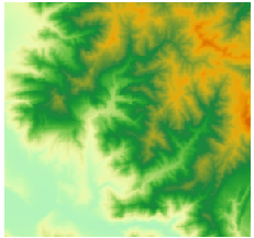
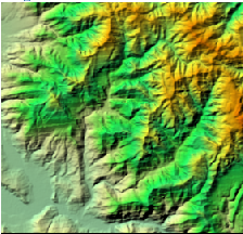
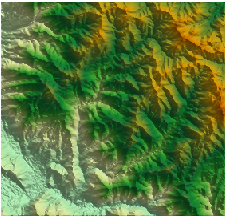
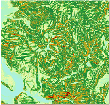
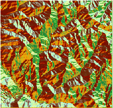
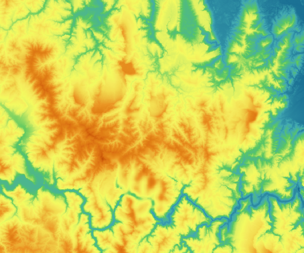
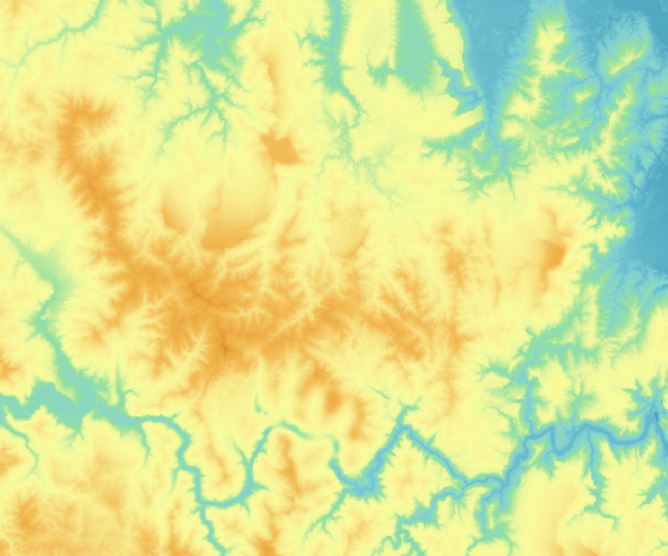
Currently, the application provides six raster function settings: 3D Hillshade, 3D Orthophoto, Slope, Aspect, Viewshed, and Terrain-RGB. These allow quick browsing of 3D hillshade effects, orthophoto effects, slope maps, aspect maps, and viewsheds without thematic analysis. The image below shows display effects of DEM data with different raster functions applied to a region.

If the map already has raster function layers, switching the dynamic projection settings (enabling or disabling) may significantly alter display effects (e.g., 3D hillshade, slope, aspect). Since the elevation scaling factor needs to adapt to the current map coordinate system, parameters should be readjusted accordingly.


Figure: Source DEM Raster Data	Figure: 3D Orthophoto	Figure: 3D Hillshade	Figure: Slope Map	Figure: Aspect Map	Figure: Viewshed

None: No raster function is applied. Settings for light source azimuth, light source elevation angle, and elevation scaling factor will be unavailable.
3D Orthophoto: Uses digital differential correction technology to correct raster data影像 by deriving reasonable sunlight intensity for the current point from surrounding raster elevations. By default, settings for light source azimuth, light source elevation angle, and elevation scaling factor are unavailable.
3D Hillshade: Generates a 3D hillshade effect by considering the angle of the illumination source and shadows on the raster surface. 3D hillshade simulates actual terrain shadows to reflect topographic relief. Using a hypothetical light source and slope aspect information from raster data, it calculates grayscale values for each cell. Slopes facing the light source have higher grayscale values, while those facing away have lower values (shadow areas), visually representing the actual地貌 and terrain. This produces a realistic 3D effect. When 3D Hillshade is selected in grid parameters, the default light source azimuth is 315 degrees, elevation angle is 45 degrees, and elevation scaling factor is 1.
Slope: Generates a slope map from DEM raster data. Default settings: light source azimuth 315 degrees, elevation angle 90 degrees, scaling factor 1.
Aspect: Generates an aspect map from DEM raster data. Default settings: light source azimuth 360 degrees, elevation angle 45 degrees, scaling factor 1.
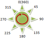
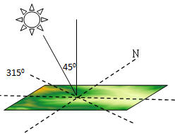
Light Source Azimuth: Determines the direction of the light source using angles. Starting from 0 degrees at true north, angles are measured clockwise from 0 to 360 degrees (true north is also 360 degrees). True east is 90 degrees, true south is 180 degrees, true west is 270 degrees. The default azimuth is 315 degrees.
Light Source Elevation Angle: The tilt angle of the light source, ranging from 0 to 90 degrees. At 90 degrees, the light shines directly downward. The default elevation angle is 45 degrees.

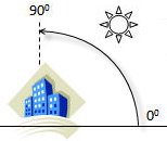
When the light source azimuth is 315 degrees and elevation angle is 45 degrees, its relationship to the surface is as shown below.
Elevation Scaling Factor: When the units of the terrain raster values (elevation) differ from the x and y coordinates, the elevation values are multiplied by a scaling factor to make the units consistent. For example, if x and y units are meters and z units are feet (1 foot = 0.3048 meters), set the scaling factor to 0.3048. A value of 1 means no scaling.
It is recommended to use projected coordinate systems (units: meters) for analysis. If using a spherical coordinate system, specify an appropriate z-factor for the latitude. If x,y units are latitude and longitude and z units are meters, use appropriate z-factors from the table below:
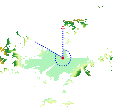
```
   Latitude     Z-factor
       0         0.00000898
      10         0.00000912
      20         0.00000956
      30         0.00001036
      40         0.00001171
      50         0.00001395
      60         0.00001792
      70         0.00002619
      80         0.00005156  
```
Viewshed: Represents the visible area from an observation point. Generate the viewshed by picking or setting the observation height and view angle range. The default view range is 360 degrees.
- X Coordinate Value: Longitude of the observation point.
- Y Coordinate Value: Latitude of the observation point.
- Altitude:: Elevation of the observation point.
- Visible Area Value: Color of the current visible area, set via the color table based on raster values.
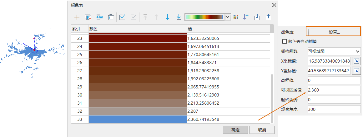
- Start Angle: Starting observation angle in degrees, measured clockwise from true north (0 degrees). Default start angle is 0.
- View Angle:: Ending observation angle in degrees, measured clockwise from true north (0 degrees). Default view angle is 360.
Terrain-RGB: Terrain-RGB is a height map format provided by Mapbox that uses RGB channels to represent elevation. The height in meters is calculated as: height = -10000 + ((R * 256 * 256 + G * 256 + B) * 0.1).
Note:
- Available only for image dataset and mosaic dataset layers when the display method is single band grid function display.
- If the color values of the image data do not represent elevation, the Terrain-RGB effect has no practical meaning.

Display Method

Provides two display methods: Combination Mode and Stretch Mode. Stretch Mode allows setting color scheme and stretch method.

Stretch methods include: Minimum Maximum, Standard Deviation, Histogram Equalization, Histogram Specification, Gaussian, and Percent Clip.

Supports batch setting of stretch methods for raster layers. Select multiple raster layers in the Layer Manager and uniformly set the stretch method in the Layer Properties panel for consistent image display effects.

Stretch Method

No Stretching: No stretching is applied to the image, but this absolute no-stretch only works effectively for unsigned 8-bit storage format image data. As shown below, the left image is an unsigned 8-bit image without stretching, appearing dark, with pixel values concentrated in lower灰度级 areas (right histogram).

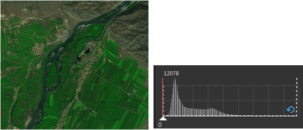
Figure: No Stretching and Histogram
Minimum Maximum: Linear stretch based on minimum and maximum values. This method uses the min and max pixel values as the range for linear stretching, distributing values between [0,255]. This enhances image contrast and brightness, making features easier to identify. Suitable for raster images with密集 pixel value distributions.
As shown below, the left image is after stretching, becoming clearer with enhanced contrast. The right histogram shows gray for before stretching and red for after.

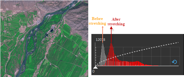
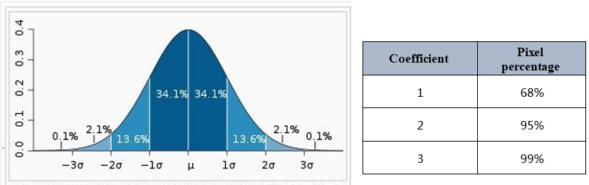
Figure: Minimum Maximum and Histograms Before/After Stretching
Standard Deviation: Enhances image contrast by trimming extreme values and linearly stretching the remaining pixels. Statistical analysis of the original image determines the one standard deviation range, which is then updated based on the standard deviation coefficient. Values within the final calculated standard deviation range are linearly stretched to [0,255], reducing the deviation of displayed pixel values from the mean.
Standard Deviation: The square root of the variance, reflecting the dispersion within a group. It indicates how much most values deviate from the mean. A larger standard deviation means greater deviation; a smaller one means values are closer to the mean.

As shown below, one standard deviation covers 68% of像素值, two cover 95%, and three cover 99%. With a standard deviation coefficient of 2, pixel values beyond two standard deviations are pushed to 0 or 255. Values within two standard deviations are linearly stretched to 0-255. Standard deviation is often used to brighten dark raster datasets.

The histogram below illustrates the standard deviation stretch method. The left image shows the effect after standard deviation stretch; the right compares histograms before and after stretching. After stretching, the histogram approximates a normal distribution curve, and the standard deviation increases, meaning pixel display values deviate less from the mean.

Standard deviation is often used to brighten dark images.

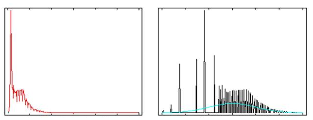
Figure: Standard Deviation Stretch and Histograms Before/After
Gaussian: Aims to make image pixel values tend towards a normal distribution. Gaussian is a linear stretch.
- Gaussian Coefficient: Pixel values are multiplied by the coefficient before stretching to [0,255].
- Using Median: If "Using Median" is checked, image stretching is performed with the median value as the central axis; if not, the maximum value is used by default.
Percent Clip: Assumes most pixels are within upper and lower limits. Set a percentage to push values outside this range to the endpoints, then linearly stretch the remaining values. This method excludes a percentage of pixels at the low and high ends from stretching, applying the minimum maximum method to the rest. Set the exclusion percentages for low and high values.
For multi-band image data, each band can be stretched separately. Click the "Histogram" button next to the combo box to open histograms for each band, specifying the minimum and maximum percentages to exclude from stretching.

Example: For an image with value range [0,100], setting min and max exclusion to 10 applies "percent clip" to stretch values between [10,90] to [0,255], while [0,10]显示为0 and [90,100]显示为255.

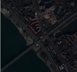
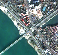
As shown below, the first image shows display effects and histogram without stretch range exclusion. The histogram shows few pixels at the extremes, affecting contrast and clarity. Excluding these pixels enhances contrast and clarity, as shown in the second image after setting the stretch range.

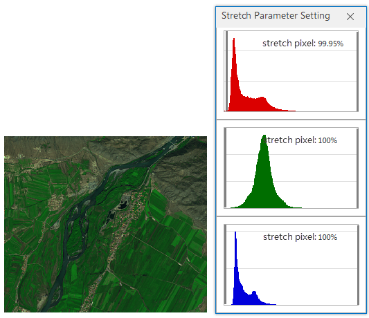
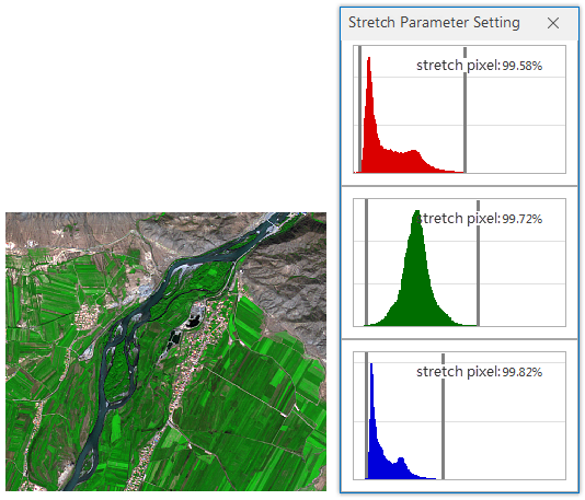
Figure 1: No Stretch Range Set Figure 2: Stretch Range Set
Histogram Equalization: A histogram modification method that non-linearly stretches the image. It redistributes pixel values to make the number of pixels大致 equal across a灰度 range, enhancing contrast in the peak areas of the original histogram while reducing it in the valleys. The output histogram is a flatter segmented histogram, enhancing image contrast.

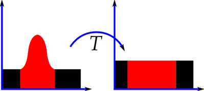
Figure: Histogram Before and After Equalization (Image Source: Internet)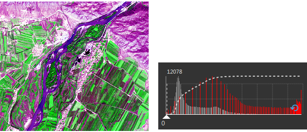

Figure: Histogram Equalization Stretch and Histograms Before/After

After histogram equalization stretch, overall image contrast is strong. The essence is trading灰度 levels for expanded contrast. This may cause loss of information at specific灰度 levels. When original remote sensing data is poor quality, has small dynamic range, or uneven histogram distribution, histogram equalization can worsen层次感 and lose more information.
Histogram Specification: Mathematically transforms the image lookup table to make its histogram resemble another image's histogram. Often used as preprocessing for adjacent image mosaicking or multi-temporal remote sensing imagery change detection. It can partially eliminate effects differences due to sun angle or atmospheric conditions.
Similar to histogram equalization, but histogram equalization has a fixed, more balanced output, while histogram specification uses an imported histogram XML file to指定 the histogram for image display.

Stretch Coefficient

Only available when the stretch method is "Standard Deviation" or "Gaussian".

Standard Deviation Coefficient: Available only when stretch method is Standard Deviation. Determines the standard deviation range. If the standard deviation range is [a,b] and the coefficient is n, the range becomes [a*n, b*n]. Default coefficient is 2, meaning 2 standard deviations are used for stretching.
Gaussian Coefficient: Available only when stretch method is Gaussian. If image pixel value range is [a,b] and the coefficient is n, Gaussian stretching keeps the central axis unchanged, stretches pixel values by n times, and displays them in [0,255]. Default coefficient is 2.

As shown below, Figure 1 is the image without any processing,整体色调偏暗, making it hard to distinguish features. After stretching (Figure 2), image contrast is enhanced, and many features become prominent.


Figure 1: Original Image	Figure 2: Stretched Image

Note:

Image stretching does not support true color 24-bit and 32-bit pixel format image data. It supports single-band and multi-band image data stretching.

Set Color Table

When the current layer is a raster layer, the Settings button can be used to set the colors of cells in the raster layer on the map. Click Settings to open the Edit Color Table dialog. Users can set the color scheme for the raster layer or assign colors to specific cell values. New cell values can be added or existing ones deleted to adjust the color display scheme for raster data. For details, see: Use and Description of the Color Table Settings Dialog.

Automatic Interpolation of the Color Chart

The automatic interpolation of the color chart function resamples raster data, optimizes raster cell boundaries, and smooths raster color effects.

Gamma

The Gamma parameter enables non-linear brightness and contrast adjustment for rasters, enhancing image display details and improving raster data display quality. Values range from 0 to 10 (inclusive), with numerical precision to two decimal places.

When Gamma = 1, no gamma correction is applied.
When Gamma > 1, contrast in dark areas increases, details become more prominent, but details in bright areas may be lost, and the overall image brightens (Figure 2).
When Gamma < 1, contrast in bright areas increases, details become more prominent, but details in dark areas may be lost, and the overall image darkens.


Figure 1: Gamma=1	Figure 2: Gamma=2