When an image layer is selected in the Layer Manager, the Layer Properties panel displays image parameter options, including brightness, contrast, transparent color, interpolation method, display method, etc.

The system supports selecting multiple image layers simultaneously for batch property settings. However, when the selected layers contain both single-band and multi-band images, you cannot uniformly set the parameters in the Display Method group.

Image Parameters

No Value Settings

• No Value: Refers to the value that has no practical meaning in the image data. You can directly enter a cell value in the text box, or click the pick-up button and pick a cell value in the image layer (snapping supported), to set the specified cell value as the No Value.
• No Value Transparent: This checkbox is used to set the display color for the specified No Value. When checked, the No Value is transparently displayed by default. When unchecked, you can click the drop-down button on the right, select a color from the popped-up color panel, and then the No Value cells of the data will be displayed in the specified color.
  Note:

  The No Value on the image dataset attribute panel is represented by an RGB decimal integer value. While the No Value on the Image Dataset Layer Properties panel is linked to the Vertex Color. When the Vertex Color is RGB, for example, if the No Value is 96555, it will be displayed as (1,21,43) in the Layer Properties panel.

Background Value Settings

The color of cells with a specified background value can be replaced with another color.

• Background Value: You can click the pick-up button and pick a cell value in the image layer on the map to set it as the background value (snapping supported). Alternatively, you can directly input a numerical value in the number box as the background value.
• Background Value Transparent: Click the drop-down button to set the replacement color in the popped-up color panel.

Transparent Color Settings

The Transparent Color setting is used to set a certain color in the image layer as transparent, meaning the area covered by the specified color in the image will be set to a transparent effect. To complete the transparent color setting, the two commands Transparent Color and Transparent Color Tolerance need to be used together.

• Transparent Color: Check this checkbox to set the specified No Value cells to transparent display; unchecking it leaves the specified No Value color displayed in its specified color. You can click the pick-up button and pick a cell color in the image layer on the map to set it as the transparent color (snapping supported). You can also click the drop-down button to select a color and set it as the transparent color.
• Transparent Color Tolerance: After setting the transparent color tolerance value, assuming the original color setting is (r, g, b) and the tolerance setting is a, the color range that needs to be transparently displayed is between (r-a, g-a, b-a) and (r+a, g+a, b+a).

Operation Steps

1. In the Layer Manager, select the image layer that needs color adjustment, and set this layer as the current layer.
2. Enable the transparent color setting for the image layer by checking the Transparent Color checkbox. Simultaneously, the color button to the right of the Transparent Color checkbox becomes available.
3. Click the drop-down button for the transparent color setting to specify the color that will have a transparent effect in the image layer.
4. Set the transparent color tolerance. You can directly input a value, or click the drop-down button on the right side of the Transparent Color Tolerance number adjustment box and use the slider to adjust the tolerance value. The transparent color tolerance is an integer between 0 and 255.
5. After the settings are complete, the image layer will immediately show the effect of the applied settings.

Brightness

When the current layer is an image layer, the Brightness number adjustment box is used to adjust the lightness and darkness of the image layer. You can directly input a brightness value in the Brightness number adjustment box to adjust the current layer's brightness. Alternatively, click the Brightness number adjustment box and use the mouse slider to adjust the brightness, viewing the result in real-time.

Contrast

When the current layer is an image layer, the Contrast number adjustment box is used to adjust the contrast of the image layer. You can directly input a contrast value in the Contrast number adjustment box to adjust the current layer's contrast. Alternatively, click the Contrast number adjustment box and use the mouse slider to adjust the contrast, viewing the result in real-time.

Image Interpolation

When zooming to browse an image layer, it's necessary to map the original image to a larger or smaller set of pixels. SuperMap provides five interpolation methods: Nearest Neighbor, Low Quality, High Quality, High Quality Bilinear Interpolation, and High Quality Bicubic. Different interpolation methods determine the display quality of the image, but the higher the output image's display quality, the longer the time required.

• Nearest Neighbor: A relatively simple image interpolation method. This method processes quickly but has the worst image display effect.
• Low Quality: This method performs pre-filtering to ensure high-quality shrinking, but the image quality when enlarged is poor after interpolation.
• High Quality: Provides high-quality image display when zooming, but takes longer to output the image.
• High Quality Bilinear Interpolation: Performs pre-filtering through the specified high-quality bilinear interpolation method to ensure high-quality display effects for scaled images.
• High Quality Bi-cubic: Performs pre-filtering through the specified high-quality bicubic method to ensure high-quality display effects for scaled images. This method outputs images with the highest display quality.

Display Method

Display Method

Based on the number of bands in the image data, it is divided into single-band and multi-band images, and the provided display method settings differ accordingly, which are introduced below. Additionally, modifying the display method is not supported for image data with a bit depth of 32 and 24.

• Single-band Image
  • Default Display: Displays the image data without stretching. If the image data has a color table, it will be displayed using the color table; if not, it will be displayed in grayscale.

    Figure: Default Display

  • Stretch Display: You can choose Minimum Maximum, Standard Deviation, Gaussian, or Percent Clip to adjust the display effect of the image, and also adjust the image's color display scheme.

    Figure: Stretch Display

  • Color Table Display: Uses the color table of the image data for display, and the color scheme can be adjusted.

    Figure: Color Table Display

• Multi-band Image
  • Combination Display: Combination display obtains color image display effects by combining multi-bands of the image according to a specified vertex color (e.g., RGB, CMYK), and supports image stretching for display settings.

    Figure: Combination Display

  • Single Band Stretch Display: Select a specific band for display, then choose a stretch method (such as Minimum Maximum, Standard Deviation, Gaussian, Percent Clip) to adjust the display effect of the image, and also adjust the image's color display scheme.

    Figure: Single Band Standard Deviation Display

  • Single Band Color Table Display: Select a specific band for display, then you can adjust the color scheme.

    Figure: Single Band Color Table Display

  • Single Band Grid Function Display: Select a specific band for display, then apply a raster function to obtain the desired display effect. For detailed information about raster functions, please refer to the Raster Function section in the raster layer properties.

    Figure: Single Band Grid Function Display

Vertex Color

Due to differences in color generation principles, there is a distinction in how devices like monitors and projectors (which directly synthesize colors using light) and printing devices like printers and presses (which use pigments) generate colors. To address these different color generation methods, SuperMap provides 7 color spaces: RGB, CMYK, RGBA, CMY, YIQ, YUV, and YCC.

The drop-down list in the vertex color combo box lists the supported color spaces, used to set the color display mode of the image data. Click the drop-down button to the right of the "color mode:" label, and select the desired vertex color from the popped-up drop-down menu to complete the vertex color setting. The default vertex color is RGB.

Vertex Color	Description
RGB	Primarily used in display systems. RGB is an abbreviation for Red, Green, Blue. The RGB vertex color assigns an intensity value in the range 0~255 to the RGB component of each pixel in the image using the RGB model.
CMYK	Primarily used in printing systems. CMYK stands for Cyan, Magenta, Yellow, and Key (Black). It mixes various colored pigments by adjusting the concentration of the three basic colors cyan, magenta, and yellow, and uses black to adjust lightness and purity.
RGBA	Primarily used in display systems. RGB is an abbreviation for Red, Green, Blue, and A is used to control transparency.
CMY	Primarily used in printing systems. CMY (Cyan, Magenta, Yellow) stands for cyan, magenta, and yellow. This type mixes various colored pigments by adjusting the concentration of the three basic colors cyan, magenta, and yellow.
YIQ	Primarily used for the North American television system (NTSC).
YUV	Primarily used for the European television system (PAL).
YCC	Primarily used for the JPEG image format.

Image Color Scheme

Layer Properties supports modifying the color scheme of image parameters. Click the combo box to the right of the label control to select a color scheme suitable for grouping. Note: To modify the image layer color scheme, the data must be a single-band image dataset with a pixel format of 8-bit or bit16. The image color scheme cannot be changed when the image layer is multi-band or composite band.

Image Stretching

During the acquisition of image data, various factors can cause some degradation in image quality. The main purpose of stretching image data is to improve its display effect and quality, thereby enhancing image clarity, highlighting certain information of interest for human or machine analysis, and suppressing some useless information to increase the practical value of the image data. Stretching image data essentially changes the brightness and contrast of the image, making features in the image easier to identify.

Currently, SuperMap provides several types of stretching for image data, including: No Stretching, Standard Deviation, Minimum Maximum, Histogram Equalization, Histogram Specification, Gaussian, and Percent Clip.

Supports batch setting of the stretch method for image layers. In the Layer Manager, select multiple image layers and uniformly set the stretch method in the Layer Properties panel, facilitating unified adjustment of image display effects.

• No stretching: No stretching processing is applied to the image. However, this absolute "no stretching" is actually only effective for image data stored in unsigned 8-bit format. The cell values displayed for image data on a computer are within the range of 0 to 255. Therefore, for image data stored in formats other than unsigned 8-bit, when displaying with "no stretch", SuperMap processes it using the Minimum Maximum method for display, making its values fall within the 0 to 255 range. As shown in the figure below, the left image shows an unsigned 8-bit image without stretching; the image appears dark. The right image is the histogram of the red band, showing cell display values concentrated in the lower gray level region.

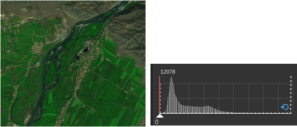
  Figure: No Stretching and Histogram

• Minimum Maximum: Refers to linear extrusion using the minimum and maximum values. This method takes the minimum and maximum cell values as the range domain and performs linear extrusion to distribute the cell values between [0,255]. Through this stretching process, the image's contrast and brightness are significantly improved, making features in the image easier to identify. It is generally suitable for stretching raster images with densely distributed pixel values.

  As shown in the figure below, the left image is the result after stretching; the image becomes clearer compared to the unstretched version, and its contrast is enhanced. The gray histogram on the right is before stretching, and the red one is after stretching.

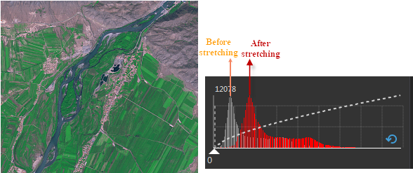
  Figure: Minimum Maximum and Histograms Before/After Stretching

• Standard Deviation: Increases the contrast of the image by clipping the image's extreme values and then performing linear extrusion on the remaining pixel values. Statistics are performed on the original image data, mainly to obtain the range of one standard deviation. Then, based on the standard deviation coefficient, the standard deviation range is updated. Finally, the values within the calculated standard deviation range are linearly extruded to distribute them between [0,255]. After stretching, the deviation of cell display values from the mean is reduced.

  Standard Deviation: The arithmetic square root of variance, reflecting the degree of dispersion among individuals within a group. Simply put, it indicates the extent to which most values in a group deviate from the average. A larger standard deviation indicates that most values deviate more from the average. A smaller standard deviation indicates that most values are closer to the average.

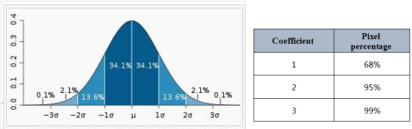
  As shown in the figure below, one standard deviation coefficient accounts for 68% of the pixel values, two standard deviation coefficients account for 95%, and three standard deviations account for 99%. When the standard deviation coefficient is defined as 2, pixel values exceeding 2 standard deviations are pushed to either 0 or 255. Pixel values within two standard deviations are linearly extruded to 0-255. 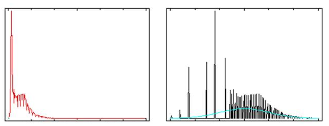Standard deviation is often used to brighten dark-toned raster datasets.

  The Standard Deviation stretch method is described visually using histograms below. As shown in the figure, the left image shows the effect after applying Standard Deviation. The right image shows a comparison of histograms before and after stretching. It can be seen that after stretching, the shape of the image's histogram approximates a normal distribution curve, and the standard deviation of the stretched image's histogram increases, meaning the deviation of cell display values from the mean is reduced.

  Standard deviation is often used to brighten dark-toned images.

  Figure: Standard Deviation Stretching and Histograms Before/After Stretching

• Gaussian: The purpose is to make the cell values of image data tend towards a normal distribution. Gaussian belongs to linear extrusion.
  • Gaussian Coefficient: The cell values of the image are multiplied by the coefficient and then stretched onto the [0,255] interval.
  • Using Median: If "Using Median" is checked, during image stretching, Gaussian stretching is performed with the median cell value as the central axis. If unchecked, it defaults to using the maximum cell value as the central axis for Gaussian stretching.
    Note:

    If the image lacks statistical information, when using Minimum Maximum, Standard Deviation, or Gaussian stretch methods, a dialog will pop up prompting "The stretch method requires statistical data information. Calculate statistics and continue?" If OK is clicked, statistics will be calculated for the image and switched to the corresponding stretch method. If Cancel is clicked, the stretch method will switch to No Stretching.

• Percent Clip: Typically, it can be assumed that most pixels in the image data are within the upper and lower limits. By setting a percentage, pixel values outside the range are pushed to the two endpoints. Then, linear extrusion is applied to the pixel values within the range. This stretch method excludes some cells from the low-value part and some from the high-value part of the histogram from the stretch, and then applies the Minimum Maximum method to the remaining part. When using it, you need to set the exclusion percentage for the minimum and maximum values.

  Stretch display can be set individually for each band of multi-band image data. You can click the "Histogram" button to the right of the combo box to open the histogram for each band, specify the minimum and maximum percentage values to be excluded from stretching, representing the percentage of cells from the low-value part and the high-value part to be excluded from stretching, respectively.

  For example: For an image with a cell value range of [0,100], defining the minimum and maximum exclusion ratios as 10 will apply "Percent Clip" to stretch values between [10,90] to the [0,255] interval for display, while [0,10] will be displayed as 0, and [90,100] as 255.

  As shown in the figure below, the first image shows the display effect and histogram without setting a stretch range. From the histogram, it can be seen that there are relatively few cells in the low-value and high-value regions, which affects the image's contrast, making it unclear. If these cells are excluded from stretching, the image's contrast and clarity can be increased. The second image below shows the effect after setting the stretch range to exclude pixels from both ends, only stretching the percentage clipped within the set range.

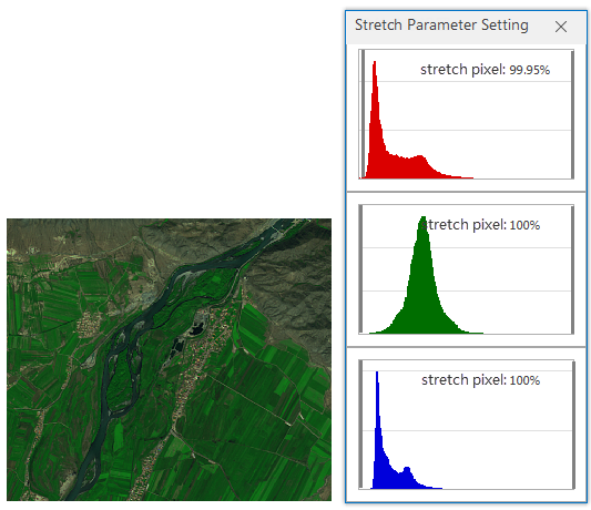
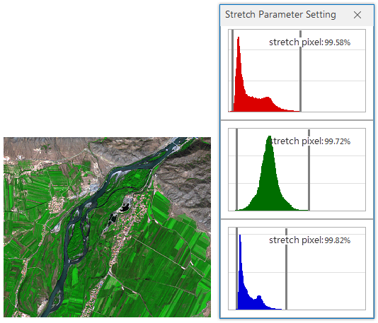
  Figure 1: No Stretch Range Set	Figure 2: Stretch Range Set

• Histogram Equalization: Belongs to the histogram modification method, essentially performing non-linear extrusion on the image. By redistributing image cell values, it makes the number of cells within a certain gray range approximately equal. This enhances the contrast of the original peak in the middle of the histogram and reduces the contrast of the valleys on both sides. The output image's histogram becomes a relatively flat segmented histogram, thereby enhancing the image's contrast.

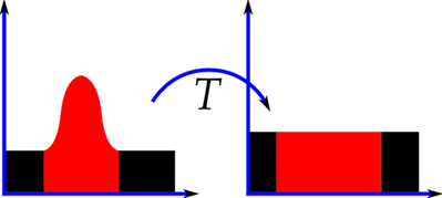
  Figure: Schematic of Image Histograms Before/After Equalization (Image Source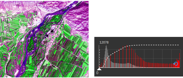: Network)

  Figure: Histogram Equalization Stretch and Histograms Before/After Stretching

  After Histogram Equalization stretching, the overall contrast of the image is strong. The essence of histogram equalization is to trade a reduction in the image's gray levels for an expansion in contrast. Therefore, sometimes when we need information at a specific gray level, that information might be lost after transformation. When the quality of the original remote sensing data is poor, the data dynamic range is small, and the histogram distribution is extremely uneven, performing histogram equalization enhancement operations may result in a transformed image with a poorer sense of hierarchy and easier loss of information.

• Histogram Specification: Performs a mathematical transformation on the image lookup table to make the histogram of one image similar to that of another. Histogram Specification is often used as a pre-processing step for adjacent image mosaicking or when using multi-temporal remote sensing imagery for dynamic change studies. It can partially eliminate differences in the effects of adjacent images caused by solar elevation angle or atmospheric influence.

  Histogram Specification is similar to Histogram Equalization, the difference being that the output result of Histogram Equalization is fixed, resulting in a more balanced image, while the result of Histogram Specification involves importing a histogram XML file and using the histogram specified by the new histogram file to display the image.

  Note:

  If an image pyramid has not been created for the image, when using Percent Clip, Histogram Specification, or Histogram Equalization, a dialog will pop up prompting "The stretch method requires creating a histogram. Create it and continue?" If OK is clicked, a histogram will be created for the image and it will switch to the corresponding stretch method. If Cancel is clicked, the stretch method will switch to No stretching.

• Adaptive stretch: Adaptive stretch (full name: Contrast Limited Adaptive Histogram Equalization) is a variant of adaptive histogram equalization. This method divides the image into multiple sub-regions, calculates the histogram for each region separately, and then redistributes the image's brightness values accordingly. This allows it to effectively enhance local contrast and improve edge clarity within each region of the image.

  However, traditional adaptive histogram equalization may excessively amplify contrast in relatively uniform areas of the image (where the histogram is highly concentrated), leading to significant noise amplification in those areas. Adaptive stretch reduces such noise amplification by limiting the degree of contrast enhancement.

  This method is suitable for enhancing the local contrast of images. It currently supports processing image data with 8-bit unsigned and 16-bit unsigned data types.

  Regarding the processing of No Value areas:

  • Specified No Value areas (typically 0 or 255): User-specified No Value areas will be identified and excluded. The pixel values in these areas retain their original values during calculation, so their display is not affected by the enhancement processing.
  • Other areas: Pixel values in areas of the image not specified as No Value will participate in the adaptive stretch calculation. After processing, these pixel values may change. If the resulting value happens to fall within the specified No Value range (e.g., 0 or 255), it may be mistakenly identified as a No Value area during display, causing visual anomalies.

  When using Adaptive Stretch, the following parameter information needs to be set:

  • Crop Threshold: By limiting the maximum number of pixels corresponding to a single pixel value in the histogram, it indirectly constrains the magnitude of local contrast enhancement. This effectively prevents significant noise amplification or artificial artifacts in noisy areas or areas with concentrated gray distributions (such as flat areas) due to over-enhancement.
  • Number of Rows/Columns for Blocking: Specifies the number of blocks into which the image is divided, i.e., total blocks = rows × columns.
    • Large number of rows/columns for blocking: Sub-region area is small, the enhancement algorithm is more sensitive to local details of the image, and local contrast improvement is more detailed and significant. However, differences in processing results between adjacent sub-regions may cause blocky boundary artifacts.
    • Small number of rows/columns for blocking: Sub-region area is large, the enhancement effect is smoother and more uniform spatially, reducing the risk of block effects. However, the enhancement effect on small-scale details and textures in the image is weakened, possibly not fully enhancing local contrast.

Gamma

The Gamma parameter enables non-linear brightness and contrast adjustment of the image, thereby enhancing image display details and improving the display quality of image data. The Gamma parameter value range is between 0 and 10 (including 0 and 10), with numerical precision to two decimal places.

• When the Gamma value equals 1, no Gamma correction is applied to the image.

• When the Gamma value is greater than 1, the contrast in the dark areas of the image increases, details become more prominent, but details in bright areas may be somewhat lost, and the overall image becomes brighter.

• When the Gamma value is less than 1, the contrast in the bright areas of the image increases, details become more prominent, but details in dark areas may be somewhat lost, and the overall image becomes darker.

Figure: Gamma=1	Figure: Gamma=2
Figure: Gamma=1	Figure: Gamma=0.4

Displays the Orthorectified Image

If the dataset associated with the layer contains RPC information, this checkbox can be enabled. Checked, it displays the orthorectified image based on elevation data; unchecked, it displays the uncorrected image.

After checking, the following three setting methods are provided in the elevation value input box and the drop-down menu on the right:

• Fixed Value: By default, displays the elevation value from the remote sensing image file. You can directly edit other values in the text input box.
• SRTM V4: Uses elevation information from the remote sensing resource package. This option is available after deploying the image environment.
• Custom: Loads elevation information by specifying DEM Data. Supports four formats: Tiff/GeoTIFF, Erdas Image, PCIDSK, and ArcInfoGrid. Among these, ArcInfoGrid format data can only be obtained by clicking the Add Folder button.

Related Topics

Set Common Layer Properties

Set Vector Layer Properties

Set Raster Layer Properties