Density Analysis

The big data distributed analysis service provides density analysis, supporting both simple density analysis and kernel density analysis methods:

Simple Density Analysis: Calculates the value per unit area within a specified neighborhood shape for each point. The resampling method divides the measurement value of each point by the specified neighborhood area. Where neighborhood areas overlap, their density values are summed. The value of each output raster represents the sum of all overlapping neighborhood density values. The unit of the result raster values is the reciprocal of the square of the original dataset unit (e.g., if the original unit is meters, the result unit becomes per square meter).
Kernel Density Analysis: Calculates the density of point and line feature measurement values within neighboring ranges to visualize the distribution of dispersed measurements across continuous areas. The result is a smooth surface with higher values at the center gradually decreasing to zero at the neighborhood boundary. This method can be used for population density analysis, building density assessment, crime report generation, tourism area monitoring, chain store performance analysis, etc.

iServer server address: Select from the dropdown to log in to the iServer address and account. For details, see the Data Input page.
Source Dataset: Set the dataset for analysis (supports line dataset and region dataset only). Click the dropdown button to select, where available datasets are automatically filtered. See Data Input for details.
Analysis Settings:

Analysis Method: Choose between simple density analysis and kernel density analysis via dropdown.
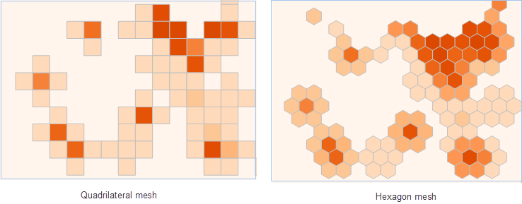
Grid Type: Required parameter. Specify quadrilateral mesh or hexagonal mesh as the grid unit. 　　
Weight Field: Optional parameter. Specify the field(s) containing weight values for points (format: col7,col8). Note: Multiple comma-separated field indices can be passed to perform multiple operations with different weights. If empty, the default weight is 1. All results are stored in the attribute table of the result dataset.
Analysis Bounds: Points outside this area are excluded from calculation. Defaults to the full extent of input data.
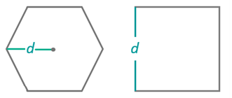
Grid Size: Side length for quadrilateral mesh or center-to-vertex distance for hexagonal mesh. Default: 50. 　　
Grid Size Unit: Options include meters, kilometers, yards, miles, feet. Default: meters.
Search Radius: Radius for density calculation. Default: 300.
Search Radius Unit: Options include meters, kilometers, yards, miles, feet. Default: meters.
Area Unit: Density denominator unit. Options: square meters, km², hectares, acres, square feet, square yards, square miles. Default: square meters.

Segmentation Mode: Includes equidistant interval, logarithmic interval, quantile interval, square root interval, standard deviation interval.
Number of Segments: Set the segmentation count for thematic maps.
Color Gradient Mode: Options include green-orange-purple gradient, green-orange gradient, rainbow, spectral gradient, terrain gradient.

Analyst Result: Execute analysis after parameter setup. Results automatically display on the map, with save paths shown in the output window. Note: Directly opening result data may fail due to server occupancy. Copy the data to another location for editing.
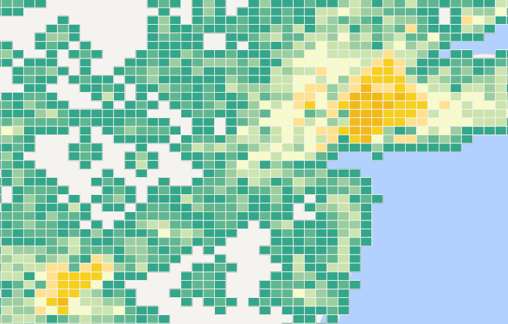
Below is a kernel density analysis result of US transaction amounts: