


The raster surface analysis function of SuperMap is based on the surface model, obtaining information or generating surfaces. It mainly includes:
Extract Contour Lines
Contour lines are one of the common methods for representing surfaces on maps. Contour lines connect adjacent points of equal value into smooth curves. Common types include elevation contours, depth contours, isotherms, isobars, and isohyets.
The distribution of contour lines reflects changes in values across the raster surface. Where contour lines are densely packed, the raster surface values change rapidly; for example, in elevation contours, denser lines indicate steeper slopes. Sparser contour lines indicate gentler changes, such as gradual slopes in elevation. Extracting contour lines helps locate positions with identical values for elevation, temperature, precipitation, etc., while their distribution reveals steep and gentle change zones.
Key Concepts
- Base Value and Contour Interval
The base value is the initial starting value for generating contour lines or surfaces. It is calculated forward or backward at intervals defined by the contour interval, so the base value may not be the minimum contour value. The base value can be any number.
The contour interval is the spacing between adjacent contour lines. Together with the base value, it determines which contour lines are extracted. For instance, with a base value of 0 and a contour interval of 50, for DEM raster data with an elevation range of 120-999, the minimum contour extracted is 150, the maximum is 950, resulting in 17 contour lines.
- Smoothness and Smoothing Method
Contour lines are generated by interpolating the original raster data and connecting points of equal value, yielding angular polylines that require smoothing to simulate real contours. Users can smooth the generated contour lines using different methods and smoothness levels.
Smoothness ranges from [0,5]. Values of 0 or 1 indicate no smoothing. Higher values increase smoothness, with 3 recommended. SuperMap offers two smoothing methods: B-spline and corner rounding. Both produce smoother contours as smoothness increases, but higher values require more computation time and memory.
SuperMap supports extracting contour lines from raster datasets via surface analysis. Three extraction methods are available: extract all isolines, extract specific isolines, and isolines from click.
- Extract All Isolines extracts all qualifying contour lines from the surface model based on specified parameters, typically controlled by the base value and contour interval.
- Extract Specific Isolines extracts contour lines at user-specified values. Users can directly input values or automatically generate a series of elevation values based on a defined range and interval.
- Isolines from Click interactively selects contour lines by clicking on the raster surface model, outputting contours equal to the clicked point's elevation value (not limited to the point's own contour).
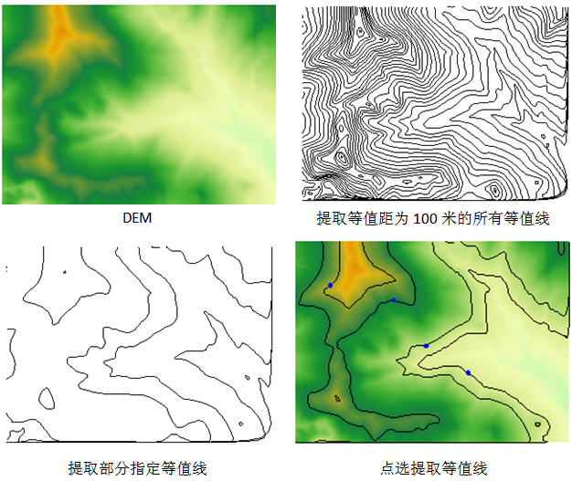
Figure: Schematic Diagram of Contour Extraction
Extract Isosurface
An isosurface is a closed surface formed by adjacent contour lines. Changes in isosurfaces visually represent variations between neighboring contours, making them effective for displaying elevation, temperature, precipitation, pollution, or atmospheric pressure. Isosurface density reflects raster surface changes: denser areas indicate larger value changes, while narrower surfaces signify steeper gradients.
SuperMap surface analysis provides two isosurface extraction methods: extract all isoregions and specified isoregions.
- Extract All Isoregions extracts all qualifying isosurfaces from the surface model based on parameters, typically the base value and contour interval. For example, with a base value of 0 and contour interval of 50, for DEM raster data ranging from 120-999, the minimum isosurface value is 150, the maximum is 950, yielding 16 isosurfaces. Isosurfaces are generated by interpolating raster data and closing adjacent contours, resulting in angular polygons that require smoothing. Smoothing methods are identical to contour lines, including B-spline and corner rounding.
- Specified Isoregions extracts isosurfaces at user-specified values. Users can input values directly or automatically generate elevation series based on a range and interval.
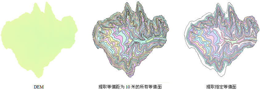
Figure: Schematic Diagram of Isosurface Extraction
Line-of-Sight
Line-of-sight, also known as visibility analysis, optimizes terrain processing. It has vital applications in navigation, aviation, and military operations, such as siting radar stations, TV transmitters, route planning, and naval navigation. Military uses include positioning defenses, setting observation posts, and laying communication lines. It also analyzes non-visible areas, e.g., low-altitude reconnaissance aircraft avoiding radar detection by flying in blind zones. Key aspects are visibility analysis between points and viewshed coverage.
A viewshed is the visible surface area from one or more observation points. It identifies regions visible from a given point on a raster dataset, based on relative height, within a specified range. The result is a raster dataset. Viewsheds are used for siting transmission towers, radar scan areas, and forest fire lookout towers.
Viewshed analysis requires key parameters: observer point, appended height, view radius, and view angle.
- Observer Point: The origin point(s) for viewshed analysis. Multiple points identify shared visible areas.
- Appended Height: The observer height combines surface elevation and appended height. For example, if a point's ground elevation is 430 meters with an appended height of 100 meters, the observer height is 530 meters.
- View Radius: This limits the viewshed search range. A radius defines a circular area centered on the observer. A default radius of 0 searches the entire map bounds.
- View Angle: This restricts the search direction in degrees (0-360), starting from north (0°) clockwise.
SuperMap supports viewshed analysis for single or multiple points. Points can be added via mouse clicks or by importing datasets. Observer points selected on the map can also be exported as point datasets.
Multi-Point Viewshed
Multi-point viewshed identifies all visible areas from multiple observer points on a raster surface, based on their relative heights. The result is a raster dataset. It can represent common viewsheds (intersection of all points) or non-common viewsheds (union).
Appended heights can be set for one or more points, significantly altering results. Multi-point viewshed allows mouse selection on raster maps or import of point datasets. Imported datasets may include elevation fields or use a uniform appended height.
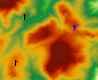
Multi-point viewshed results are shown below:
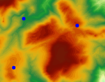 |
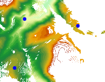 |
| DEM Dataset and Observation Points | Multi-Point Viewshed Result |
Visibility analysis determines if points are mutually visible on a raster surface. SuperMap offers two-point and multi-point visibility analysis based on observer count.
- Two-Point Visibility analyzes mutual visibility between any two surface points.
Since DEMs lack above-ground features like trees or buildings, appended heights adjust observer elevations for accuracy. Omitting appended heights may yield opposite results. Two-point analysis can be done via mouse clicks or imported point datasets.
- Multi-Point Visibility analyzes pairwise visibility among multiple points on a raster surface.
Appended heights can be set per point, potentially reversing results. Points can be selected via mouse or imported datasets.
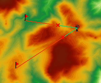
DEM Dataset and Observation Points Multi-Point Visibility Analysis Result 3D spatial analysis enhances 2D functions with intuitive visualization. Below shows multi-point visibility in a scene.
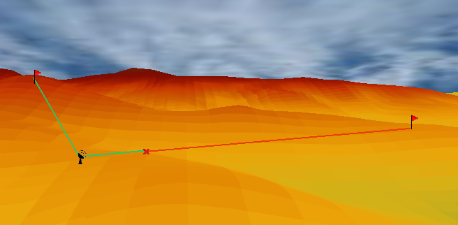
Multi-Point Visibility Effect in 3D Scene
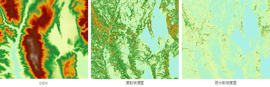
Slope and Aspect
Slope and aspect are crucial terrain factors in surface analysis. Slope measures the rate of elevation change, while aspect indicates the direction of slope change.
Slope analysis is essential for tasks like finding flat areas for construction, selecting ski slopes of varying difficulty, identifying landing zones for rescue aircraft, or enforcing farmland slope restrictions (e.g., no cultivation above 25°).
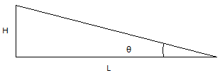
Slope at a point is a vector with magnitude and direction, defined as the angle between the tangent plane and horizontal surface. Slope maps show terrain steepness, with higher values indicating steeper slopes. Slope can be expressed in degrees, radians, or percentages. For vertical increment H and horizontal increment L, degree slope: θ = arctan(H / L), radian slope: R = θ * π / 180, percentage slope: P = (H / L) * 100.
 |
Degree slopes range from 0° (horizontal) to 90° (vertical). Percentage slopes range from 0 to infinity: values below 1 indicate gentle slopes, 1 equals 45°, and above 1 indicate steeper slopes. Raster datasets (GRID) calculate average slope per cell plane by interpolating elevations.
 |
Aspect is vital in vegetation analysis, environmental assessment, wind farm siting, geological studies, and snowmelt hazard identification. For example, north- and south-facing slopes support different vegetation due to sunlight exposure.
Aspect at a point is the direction of maximum elevation change, measured in degrees from north (0°) clockwise to 360°. Flat areas have an aspect of -1.
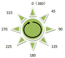 |
Since aspect is circular (e.g., 10° is closer to 360° than 30°), users should reclassify it into cardinal directions (e.g., 4 or 8 directions) using raster reclassification to highlight relevant ranges.
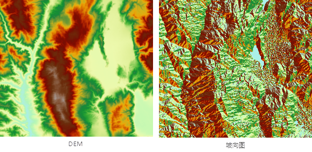 |
Surface Cut Fill
Surface cut fill quantifies material movement due to erosion or deposition, where "cut" denotes removal and "fill" denotes addition. It calculates the area and volume needed to transform one state to another, as shown in the terrain profile below.
 |
Raster cut fill requires two input raster datasets: pre-cut/fill and post-cut/fill. The result dataset has cell values equal to the difference (pre minus post). Positive values indicate cut (material removal), negative values indicate fill (material addition). A 4x4 raster example illustrates the calculation:
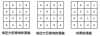 |
Result dataset = pre-cut/fill raster dataset - post-cut/fill raster dataset.
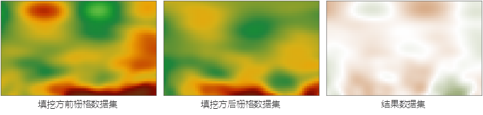
The diagram below shows source data, reference cut fill data, and the result. In the result, cut areas are dark green (darker for larger volumes), fill areas are brown (darker for larger volumes), and unchanged areas are white.
 |
Input datasets must share the same coordinate and projection systems to ensure correct location matching. Mismatched systems may cause errors. Only overlapping areas are processed if spatial ranges differ, and null cells in either input yield null results. The result dataset's extent matches the overlap area.
Surface cut fill computes cut/fill volumes between a raster dataset and a specified plane, which can be an existing vector dataset or a drawn region. This is broader and more flexible than standard cut fill, which compares two rasters.
Inverse cut fill calculates post-cut/fill elevation from a base raster and a given cut/fill volume. It addresses real-world problems like determining the final elevation after adding a known soil volume. For example, if a construction site requires fill and a source provides volume V, inverse cut fill computes the resulting elevation to assess if additional fill is needed.