


Ordinary Least Squares (OLS) is the simplest and most widely used regression method. OLS provides a global model for the variable or process that users want to understand/predict, creating a single regression equation to represent the process. Geographically Weighted Regression (GWR), as one of several spatial regression methods, is increasingly used in geography and other disciplines. By fitting regression equations to each feature in the dataset, GWR provides a local model for the variable or process under study.
Feature Entry
- Spatial Statistics Tab -> Spatial Relationship Modeling -> Ordinary Least Squares (OLS).
- Toolbox->Spatial Statistics->Spatial Relationship Modeling ->Ordinary Least Squares (OLS).
Parameter Description
- Source Dataset: Specifies the vector dataset to analyze, supporting point, line, and polygon datasets. Note: The object count in the source dataset must be greater than 3.
- Explanatory Variables: Explanatory variables are independent variables (X on the right side of the regression equation). Select one or more numeric fields as explanatory variables to model or predict the dependent variable. Note: If all values of an explanatory variable are equal, the OLS regression equation cannot be solved.
- Dependent Variable: The variable to be studied or predicted (Y on the left side of the regression equation), supporting only numeric fields. The regression model is built based on known observations to predict the dependent variable.
- Result Data: Specifies the datasource and dataset name for storing results, with data type consistent with the source data.
Result Output
The predicted values, residuals, and standardized residuals from OLS analysis are recorded in the property fields of the result dataset. Statistical results such as distribution statistics, probability values, AICc, and coefficient of determination are displayed in the OLS report. The analysis results are described as follows:
Results in Attribute Table
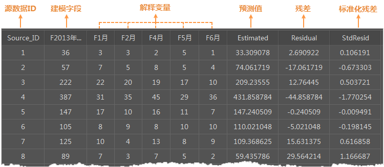
- Source_ID: The SmID value from the source dataset, serving as the unique identifier.
- Dependent Variable and Explanatory Fields: Retains original dependent and explanatory fields from the source data.
- Estimated (Predicted Value): Fitted values obtained through OLS analysis based on specified explanatory variables.
- Residual: Unexplained portion of the dependent variable, calculated as the difference between estimated and actual values. The mean of standardized residuals is 0 with a standard deviation of 1. Smaller residuals indicate better model fit. Spatial autocorrelation analysis of residuals may reveal missing key variables if high/low residuals show statistically significant clustering, making OLS results unreliable.
- StdResid (Standardized Residual): Ratio of residual to standard error. Values within (-2, 2) suggest normality and homoscedasticity. Values outside this range indicate outliers or non-normality. Non-normal distributions suggest model bias, possibly due to missing variables.
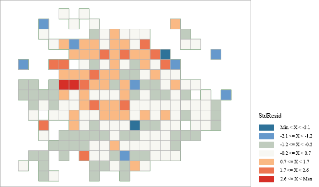
Visualization of Model Residuals
A graduated color thematic map of residuals is generated after analysis. A valid regression model shows randomly distributed over/under-predictions. Clustered residuals indicate missing key explanatory variables. Performing Hot Spot Analysis (Getis-Ord Gi*) on residuals can help identify spatial patterns.
OLS Report
The output window displays an OLS report containing detailed analysis results, including model variables, significance tests, variable distributions, standardized residual histograms, and residual-prediction scatter plots:
- Model Variables
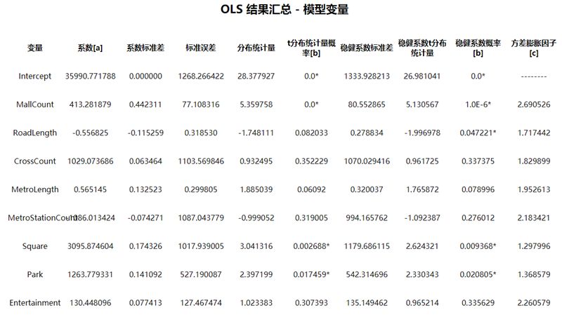
- Coefficient: Reflects relationship strength and direction between each explanatory variable and the dependent variable. Larger absolute values indicate greater contribution. Positive/negative signs denote positive/negative correlations.
- Coefficient Standard Errors: Measures dispersion of coefficient estimates. Smaller values indicate higher reliability.
- Distribution Statistic: Evaluates statistical significance of explanatory variables (t-Statistic = mean / standard error). Larger values indicate higher significance.
- Probability: A small p-value (e.g., <0.05) indicates the coefficient is statistically significant.
- Robust Coefficient Standard Errors: Assesses coefficient stability when variables are modified.
- Robust Coefficient Probability: Used when Koenker (Breusch-Pagan) statistic is significant.
- Variance Inflation Factor (VIF): Values exceeding 7.5 suggest redundant variables (multicollinearity).
- Model Significance
- AIC: Balances model complexity and goodness-of-fit. Lower values indicate better models.
- AICc: Adjusted AIC for small sample sizes. Models with AICc differences >3 are considered significantly different.
- Coefficient of Determination (R²): Proportion of variance explained by the model (0.0-1.0). Higher values suggest better fit.
- Adjusted R²: Compensates for model complexity. Generally lower than R² but more reliable for model comparison.
- Joint F-Statistic: Tests overall model significance when Koenker statistic is insignificant.
- Joint Chi-Square Statistic: Tests model significance when Koenker statistic is significant.
- Koenker (Breusch-Pagan) Statistic: Tests model stability (homoscedasticity). Significant p-values (<0.05) indicate non-stationarity.
- Jarque-Bera Statistic: Tests residual normality. Significant p-values suggest model bias.
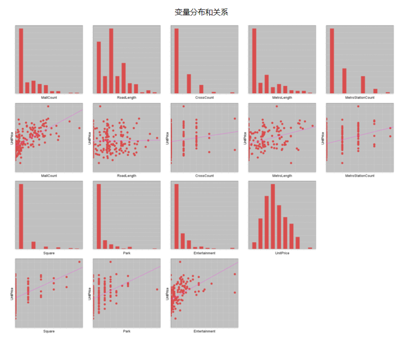
- Variable Distribution and Relationship
Histograms show variable distributions. Scatter plots visualize relationships between explanatory variables and the dependent variable. Strong linear relationships appear diagonal.
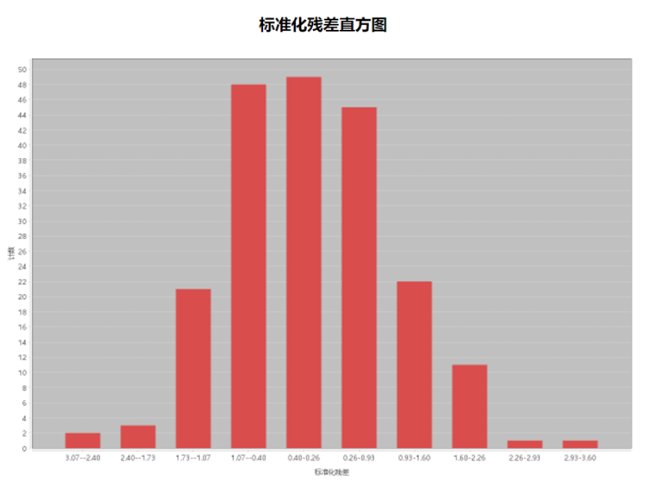
- Standardized Residual Histogram
Ideal residual distribution should approximate normality. Significant deviations indicate model bias.
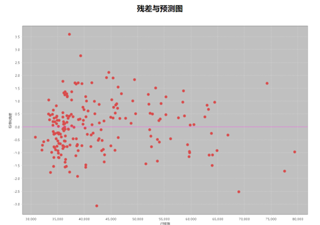
- Residual vs Prediction Graph
Scatter plot shows heteroscedasticity. Systematic patterns indicate prediction accuracy varies across values.
Model Evaluation
After selecting variables and performing OLS analysis, evaluate model validity using these criteria:
- Variable Significance
- Absolute coefficient magnitude indicates contribution size.
- p-values <0.05 indicate statistical significance.
- Use robust probabilities when Koenker statistic is significant.
- Variable Relationships
Coefficient signs should match expected theoretical relationships. Unexpected signs may reveal missing variables.
- Redundant Variables
VIF >7.5 suggests redundancy. Remove redundant variables unless the model performs well for prediction.
- Model Bias
Check residual normality. Non-normal distributions may require variable transformations (log/exponential) or outlier removal.
- Missing Key Variables
Statistically significant spatial autocorrelation in residuals (p<0.05) indicates missing variables.
- Model Performance
Adjusted R² values (0-1) indicate explained variance percentage. AICc values help compare models, with lower values preferred.
Related Topics
Geographically Weighted Regression (GWR)
Measuring Geographic Distributions