


Geographically weighted regression (GWR) is a recently developed spatial analysis method that serves as a local regression model. It detects spatial non-stationarity by embedding spatial structures into linear regression models. Through regression analysis, we can model, examine, and explore spatial relationships, interpret factors behind observed spatial patterns, and make predictions.
For principles and application scenarios, see the Regression Analysis page.
Feature Entry
- Spatial Statistics Tab -> Spatial Relationship Modeling -> Geographically Weighted Regression (GWR).
- Toolbox->Spatial Statistics->Spatial Relationship Modeling ->Geographically Weighted Regression (GWR).
Parameter Description
- Source Dataset: Specifies the vector dataset to analyze, supporting point, line, and polygon datasets. Note: The object count must exceed 20.
- Explanatory Fields: Explanatory variables (independent variables X in regression equations) model or predict dependent variables. For example, in studying obesity causes, variables like income, healthy food intake, and education level would be explanatory variables (X), while obesity is the dependent variable (Y).
- Kernel Function Type: Defines distance weight calculation between points. Five kernel types are supported. Formulas use: W_ij as weight between points i and j; d_ij as distance; b as bandwidth.
- Quadratic kernel: W_ij=(1-(d_ij/b)^2)^2 if d_ij≤b; otherwise W_ij=0.
- Boxcar kernel: W_ij=1 if d_ij≤b; otherwise W_ij=0.
- Gaussian kernel: W_ij=e^(-((d_ij/b)^2)/2).
- Tricube kernel: W_ij=(1-(d_ij/b)^3)^3 if d_ij≤b; otherwise W_ij=0.
- Dependent Field: The studied/predicted variable (Y), supporting numeric fields only.
- Bandwidth Method: Determines bandwidth selection:
- Akaike Information Criterion (AICc): Recommended when unsure about distance or neighbor count parameters.
- Cross-validation (CV): Excludes regression points themselves during coefficient estimation. CV score reflects squared differences between estimated and actual values.
- Fixed distance/neighbors: Requires specifying exact distance or neighbor count.
- Bandwidth Type:
- Fixed bandwidth: Requires setting "Bandwidth" value when using fixed distance method. Automatically calculated for AICc/CV methods.
- Variable bandwidth: Requires "Neighbor Count" when using variable distance method. Automatically finds neighbors for AICc/CV methods.
- Prediction Item: Enables predictions using GWR results.
- Prediction data settings: Specifies output datasource and dataset name.
- Field mapping: Ensures correspondence between prediction and source dataset fields. Mandatory if prediction dataset lacks source explanatory fields.
- Prediction result settings: Defines output datasource and dataset name for prediction results.
- Result Settings: Specifies output datasource and dataset name.
Result Output
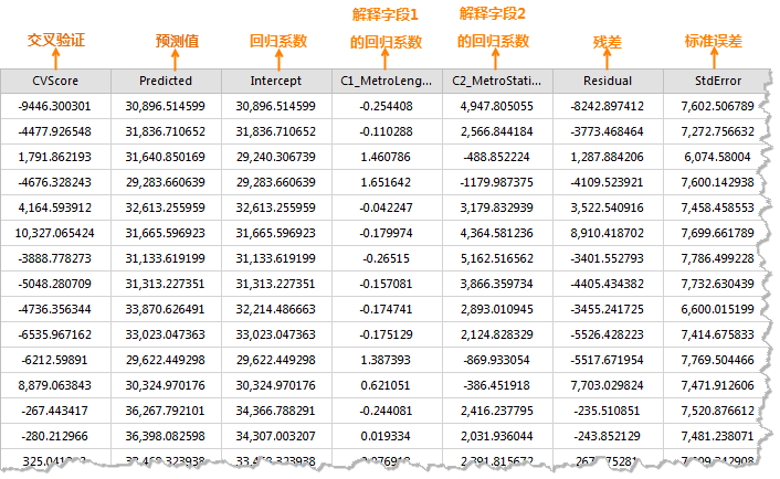
After parameter setup, click "OK" to execute GWR. Result datasets contain fields: CVScore, Predicted, Intercept, C1_explanatory field names, Residual, StdError, SE_Intercept, SE1_explanatory field names, TV_Intercept, TV1_explanatory field names, and StdResidual. Example:
-
CVScore: Sum of squared differences between cross-validated estimates and actual values, serving as model performance metric.
-
Predicted: Estimated values from GWR.
-
Intercept: Regression intercept when all explanatory variables equal zero.
-
C1_explanatory field names: Regression coefficients indicating relationship strength/direction. Positive values denote positive correlations.
-
Residual: Unexplained variance (difference between predicted and actual values). Smaller residuals indicate better model fit.
-
StdError: Estimates reliability metric. Smaller values suggest better precision.
-
SE_Intercept/SE1_explanatory field names: Coefficient reliability indicators. Large values may suggest multicollinearity.
-
TV_Intercept/TV1_explanatory field names: Coefficient significance tests. Values exceeding critical thresholds indicate statistical significance.
-
StdResidual: Residual-to-StdError ratio. Values within (-2, 2) suggest normality; outliers indicate anomalies.
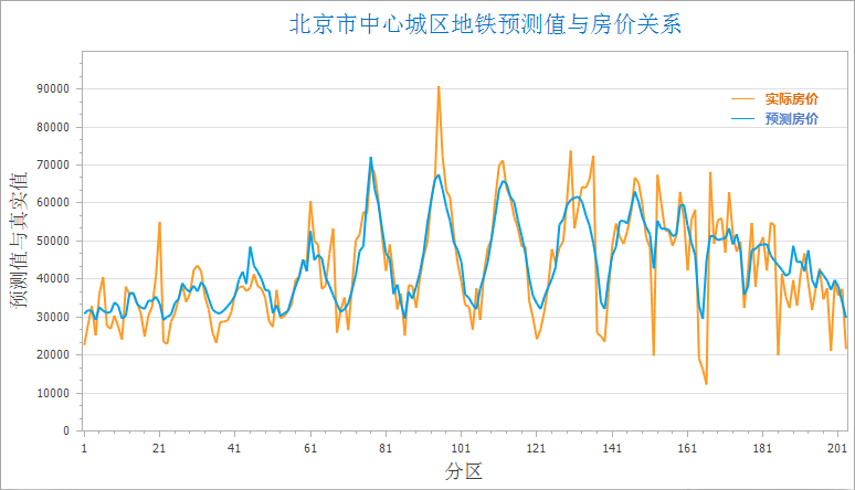
The figure below compares actual vs predicted housing prices in central Beijing (2016), using subway station count and line length as explanatory variables. Orange lines represent actual values, blue lines show fitted values.
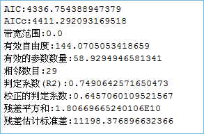
Upon successful execution, the output window displays analysis results (shown below). If residuals are acceptable, use the model for predictions.
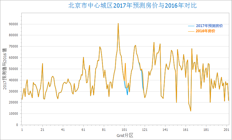
Using 2017 subway expansion data, predicted housing prices are calculated as: 2017 Price = Intercept + C1*(2017 stations) + C2*(2017 line length). The figure shows price fluctuations in areas with subway changes.
Related Topics
Measuring Geographic Distributions