


Hot Spot Analysis is given a set of weighted features, identifies statistically significant hot spots and cold spots using the Getis-Ord Gi* statistic. Hot Spot Analysis (Getis-Ord Gi*) examines each feature within the context of neighboring features. A single isolated high value does not constitute a hot spot; a true hot spot requires both the feature itself and its surrounding features to be high-value clusters. Conversely, a cold spot indicates not only low values of the feature itself but also adjacent low-value aggregations.
Application examples
Application fields include: crime analysis, epidemiology, voting pattern analysis, economic geography, retail analysis, traffic accident analysis, and demographics. Some specific examples:
- Where are disease outbreaks concentrated?
- Where do kitchen fires account for an abnormally high proportion of residential fires?
- Where should emergency evacuation zones be located?
- Where/when do peak density areas occur?
- Where and during which periods should additional resources be allocated?
Feature entry
- Spatial Statistics Tab -> Cluster Distribution -> Hot Spot Analysis (Getis-Ord Gi*).
- Toolbox->Spatial Statistics->Cluster Distribution->Hot Spot Analysis (Getis-Ord Gi*).
Parameter Description
- Result settings: Specifies output datasource and dataset name.
Result interpretation
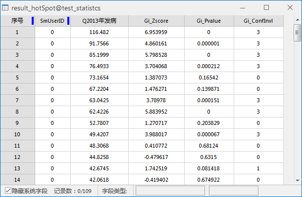
The result dataset contains three fields: Z-score (Gi_Zscore), P-value (Gi_Pvalue), and confidence interval (Gi_ConfInvl). Results are rendered by Gi_ConfInvl values on maps, with evaluation field histograms in statistical charts:
| Z score (SD) | Interpretation | Hot spot/Cold spot |
|---|---|---|
| Z>0 with small P | High-value spatial cluster. Higher Z indicates stronger clustering. | Hot spot (positive Gi_ConfInvl) |
| Z ≈ 0 | No significant clustering | -- |
| Z<0 with small P | Low-value spatial cluster. Lower Z indicates stronger clustering | Cold spot (negative Gi_ConfInvl) |
Detailed value mapping:
| Z score | P value | Gi_ConfInvl | Confidence | Result interpretation |
|---|---|---|---|---|
| <-2.58 | <0.01 | -3 | 99% | Cold spot with 99% confidence |
| < -1.96 | < 0.05 | -2 | 95% | Cold spot with 95% confidence |
| <-1.65 | <0.1 | -1 | 90% | Cold spot with 90% confidence |
| ≈0 | -- | 0 | -- | Statistically insignificant |
| >1.65 | <0.1 | 1 | 90% | Hot spot with 90% confidence |
| >1.96 | < 0.05 | 2 | 95% | Hot spot with 95% confidence |
| >2.58 | <0.01 | 3 | 99% | Hot spot with 99% confidence |
Case study
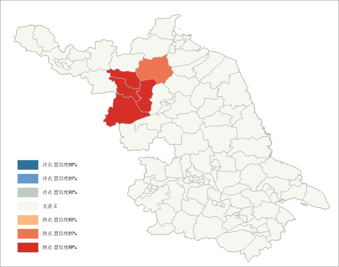
Analyzing 2013 viral hepatitis incidence using Hot Spot Analysis (Getis-Ord Gi*). Parameters: evaluation field=2013 case count, conceptualization=inverse distance, measure method=Euclidean distance, standardized spatial weight matrix. Results:
Under random distribution assumption:
- Red areas in northwest show Z>2.58, indicating high-value clusters surrounded by high values. Approximately 5 regions exhibit significant hot spots requiring preventive measures.
- Gray-white areas (Z≈0) show no statistical significance.
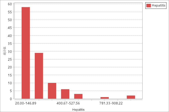
Case count histogram:
Related Topics
Cluster and Outlier Analysis (Anselin Local Moran's I)