


Cluster and Outlier Analysis can be used to identifies statistically significant hot spots, cold spots, and spatial outliers using the Anselin Local Moran's I statistic.
A scatter plot is a common method in data analysis to represent the correlation between two variables. To represent the spatial autocorrelation relationship of a variable, the Moran scatter plot can be used.
Moran Scatter Plot
The Moran scatter plot can be used to explore global patterns of spatial association, identify spatial anomalies and local non-stationarity. By plotting the observed values of a variable on the x-axis and their spatial lags (standardized local spatial autocorrelation index Moran's I) on the y-axis, the correlation between them is visually represented in the coordinate system.
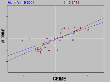
- The Moran scatter plot is divided into four quadrants, corresponding to four different types of local spatial association patterns:
- Upper-right quadrant (H-H): The observed value zi is above the mean (high), and its spatial lag is also above the mean (high).
- Lower-left quadrant (L-L): The observed value zi is below the mean (low), and its spatial lag is also below the mean (low).
- Upper-left quadrant (L-H): The observed value zi is below the mean (low), but its spatial lag is above the mean (high).
- Lower-right quadrant (H-L): The observed value zi is above the mean (high), but its spatial lag is below the mean (low).
- Interpretations of spatial relationships in different quadrants:
- Upper-right (H-H) and lower-left (L-L) quadrants indicate positive spatial autocorrelation, representing similarity between observed values at a location and its neighboring locations. Specifically, H-H corresponds to high-high similarity and L-L corresponds to low-low similarity.
- Upper-left (L-H) and lower-right (H-L) quadrants indicate negative spatial autocorrelation, representing dissimilarity between observed values at a location and its neighbors. L-H corresponds to low-high dissimilarity, while H-L corresponds to high-low dissimilarity, where low values are surrounded by high values or vice versa.
- The H-H and L-L quadrants correspond to positive spatial associations (high-high) and negative spatial associations (low-low) in the G statistic. Observing the relative density of these quadrants reveals the dominance of high-value or low-value associations in global spatial patterns.
- Observing the relative density of L-H and H-L quadrants helps identify which form of negative spatial association predominates.
- Additionally, potential spatial outliers can be detected by drawing a circle with radius 2 centered at the origin of the scatter plot. Points outside this circle (2 standard deviations from the mean) are considered outliers since the plot uses standardized variables and their spatial lags.
- When displaying only statistically significant high or low observations in the Moran scatter map, a Moran significance map is generated. Significant observations in the first or third quadrants indicate spatial clustering, while those in the second or fourth quadrants indicate spatial dissimilarity.
Application Cases
- Identifying the clearest boundaries between affluent and impoverished areas in a study region.
- Locating areas with anomalous consumption patterns.
- Detecting unexpected high-incidence areas of diabetes.
Feature Entry
- Spatial Statistics Tab ->Cluster Distribution->Cluster and Outlier Analysis (Anselin Local Moran's I).
- Toolbox->Spatial Statistics->Cluster Distribution->Cluster and Outlier Analysis (Anselin Local Moran's I).
Main Parameters
- Source Dataset: Specifies the vector dataset to analyze, supporting point, line, and polygon datasets.
- Evaluation Field: Specifies the numeric field containing values for analysis.
- Conceptualization Model: Choose a model reflecting inherent relationships between features. More realistic models yield more accurate results.
- Fixed distance: Suitable for point data or polygon data with highly variable sizes.
- Polygon adjacent (common edges/intersect): Suitable for polygons sharing edges or intersections.
- Polygon adjacent (node/common edges/intersect): Suitable for polygons sharing nodes, edges, or intersections.
- Inverse distance: All features influence each other, with weights inversely proportional to distance. Suitable for continuous data.
- Inverse distance square: Similar to "inverse distance" but with faster weight decay (inverse square of distance).
- K Nearest Neighbors: Only the nearest K features to the target are included (weight=1). Effective for ensuring minimum neighbors and handling spatially varying data distributions.
- Spatial weight matrix: Requires a spatial weight matrix file (.swmb) modeling network-based relationships (e.g., road network distances). Useful for accessibility studies.
- Undifferentiated region: Combines "inverse distance" and "fixed distance." Features within a threshold distance have equal weights (weight=1), while others follow inverse distance decay.
- Distance Threshold: "-1" computes a default distance ensuring each feature has at least one neighbor; "0" treats all features as neighbors; positive values define adjacency distance.
- Inverse Distance Power: Exponent controlling distance decay effect (higher values diminish distant influences faster).
- Number of Neighbors: Positive integer specifying the K nearest neighbors.
- Measure Distance Method: Euclidean distance or Manhattan distance. For details, see Spatial Statistics Basic Vocabulary.
- Spatial Weights Matrix Standardization: Recommended when sampling bias exists. Weights are divided by row sums, creating relative weights (0-1). Essential for polygon adjacency analyses and administrative boundaries.
- Apply FDR Correction: If enabled, statistical significance uses False Discovery Rate correction; otherwise, it uses raw p-values and Z-scores.
Result Interpretation
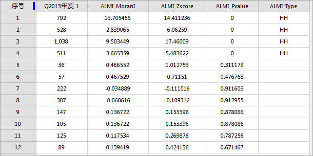
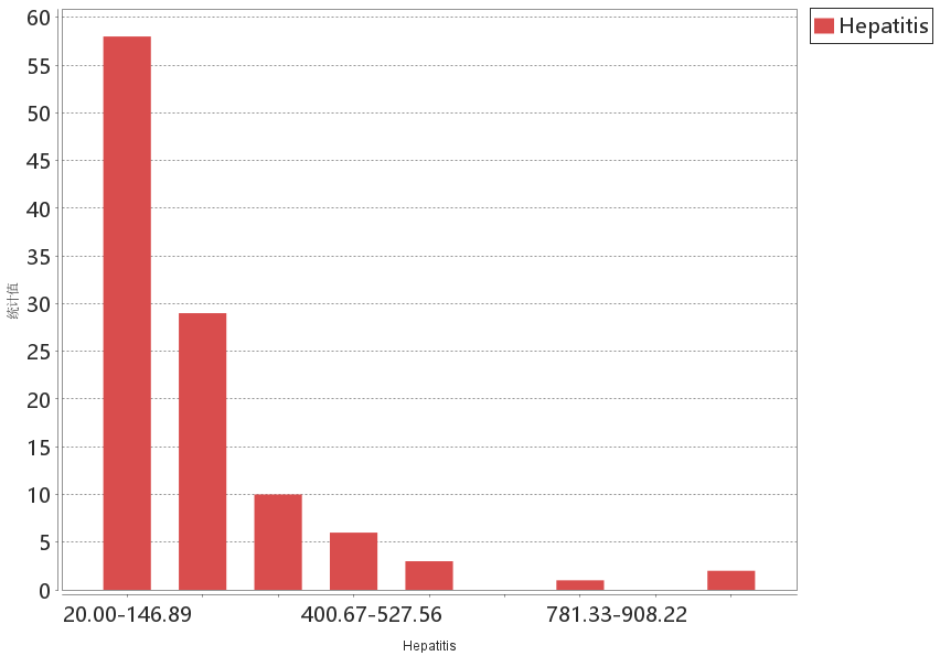
The output is a region dataset containing four fields: ALMI_MoranI (local Moran's I), ALMI_Zscore, ALMI_Pvalue, and ALMI_Type (cluster/outlier type). The map renders ALMI_Type values, while the histogram displays the evaluation field distribution. Key points:
Clusters and outliers are calculated at 95% confidence. ALMI_Type values exist only when p-value <0.05. If FDR correction is applied, significance thresholds are adjusted for multiple testing.
| P-value (ALMI_Pvalue) | Moran's I (ALMI_MoranI) | Interpretation | Cluster/Outlier Type (AIMI_TYPE) |
|---|---|---|---|
| P < 0.05 | M > 0 | High-value or low-value cluster | HH (High-High) or LL (Low-Low) |
| P < 0.05 | M < 0 | Outlier | HL (High-Low) or LH (Low-High) |
| P-value (ALMI_Pvalue) | Z-score (ALMI_Zscore) | Interpretation | Cluster/Outlier Type (AIMI_TYPE) |
|---|---|---|---|
| P < 0.05 | Z > 0 | Similar surrounding values (high or low) | HH or LL |
| P < 0.05 | Z < 0 | Statistically significant spatial outlier | HL or LH |
Example
Sample Data: Click to download ClusterDistributions Sample Data (extract after download).
Performing cluster and outlier analysis on 2013 pneumonia incidence data at county level: Set evaluation field to "2013 Cases", conceptualization model to inverse distance, measure distance method to Euclidean, enable spatial weights standardization and FDR correction. Result dataset attributes are shown below:
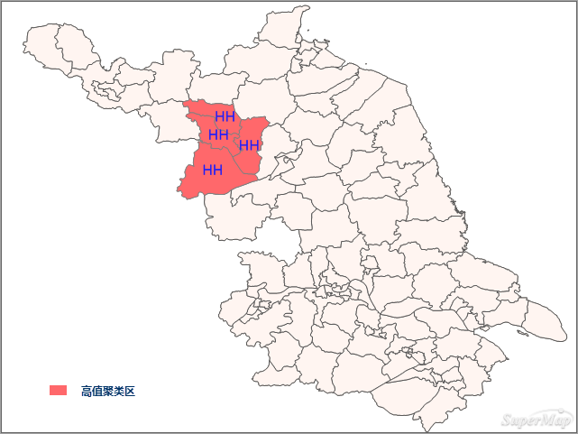
Under random distribution assumption:
- Red areas in the northwest show significant Z-scores, indicating high-value spatial clustering.
- HH regions (high-high clusters) suggest both local and neighboring areas have high incidence, requiring medical vigilance.
Most regions show insignificant Moran's I values, with significant areas predominantly high-high clusters.
Histogram of incidence data:
Related Topics
Hot Spot Analysis (Getis-Ord Gi*)