


Interpolation uses known sample points to predict or estimate the values of unknown sample points. Interpolation refers to estimating unknown point data within the same region based on known point data. Extrapolation involves estimating data in other regions based on known regions. Both interpolation and extrapolation are common concepts in the interpolation process. SuperMap provides three interpolation methods for simulating or creating a surface: Inverse Distance Weighted (IDW), Kriging, and Radial Basis Function (RBF). The choice of interpolation method usually depends on the distribution of sample data and the type of surface to be created. Regardless of the interpolation method chosen, the more known data points there are and the wider their distribution, the closer the interpolation results will be to the actual situation.
Inverse Distance Weighted (IDW) Interpolation
Inverse Distance Weighted (IDW) interpolation is based on the principle that points closer together are more similar. It estimates cell values by calculating the weighted mean of nearby sample points, with closer points having higher weights. This is a simple and effective data interpolation method with relatively fast computation speed.
Besides weight distance, power and search radius are also key factors influencing IDW interpolation.
- Power: Related to the calculation of weight distance, the power exponent significantly affects IDW interpolation results. Lower power values yield smoother results, while higher values provide more detailed outcomes. The default power is 2.
- Search radius: There are two types of search radius for IDW interpolation:
- Fixed count: A specified number of nearest sample points to the raster cell participate in interpolation. The number of sample points is fixed for each cell, but the search radius varies based on local point density. Sample points beyond the maximum search range are excluded.
- Fixed radius: All sample points within a specified radius participate in interpolation. If the number falls below the minimum threshold, the radius expands to include more points.
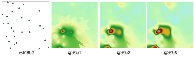
The figure below shows surface interpolation effects using IDW with elevation as the interpolation field, resolution of 100, fixed count search radius (all points included), and power values of 1, 2, and 3.
Spline Interpolation
Spline functions mathematically mimic manual splines to draw smooth curves through sample points. Spline interpolation is a precise technique that assumes smooth changes, featuring two characteristics: (1) the surface must pass exactly through all sample points, and (2) the surface must have minimal curvature. It excels in creating visually smooth curves and contours.
Spline interpolation is suitable for interpolating large sample sets while requiring smooth surfaces. It performs well under gentle surface changes but is unsuitable for abrupt value shifts over short horizontal distances or with inaccurate sample data.
Spline interpolation offers three search radius types:
- Fixed count: A specified number of nearest sample points to the raster cell participate in interpolation. The number is fixed, but the search radius varies with local density. Points beyond the maximum range are excluded.
- Fixed radius: All sample points within a specified radius participate. The radius expands if points fall below the minimum threshold.
- Block search: Divides the dataset into blocks based on maximum points per block, using points within each block for interpolation.
Kriging Interpolation
Kriging interpolation, based on spatial autocorrelation, uses variogram models for unbiased estimation of unknown points within a limited area. It is optimal when sample points exhibit spatial autocorrelation or directional trends. Spatial autocorrelation implies interdependence among sample points within a region, with stronger correlations for closer points. Kriging is widely used in soil science and geology.
SuperMap supports three semi-variogram models: spherical, exponential, and Gaussian.
Semi-variogram models characterize spatial autocorrelation, described by range, sill, and nugget effect.
- Semi-variogram model

Figure: Spherical model diagram 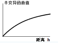
Figure: Exponential model diagram 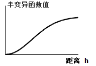
Figure: Gaussian model diagram - Spherical model shows spatial autocorrelation decreasing gradually (semi-variogram increasing) until correlation vanishes beyond a certain distance. It is commonly used.
- Exponential model applies when spatial autocorrelation decreases exponentially with distance. It is frequently employed.
- Gaussian model suits scenarios where semi-variogram values asymptotically approach the sill.
- Parameter description
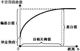
Figure: Range, sill, and nugget effect diagram - Range: The distance where semi-variogram values stabilize. Within this range, sample points are correlated; beyond it, they are independent and do not affect estimation.
- Sill: The peak value of the semi-variogram. Sill minus nugget effect gives the partial sill.
- Nugget effect: The value where semi-variogram intersects the Y-axis at h=0, indicating micro-scale variability due to measurement errors or mineralization.
SuperMap provides three Kriging methods: ordinary kriging, simple kriging, and universal kriging.
- Ordinary kriging: A linear estimator assuming normally distributed data with an unknown mean for the regionalized variable.
- Simple kriging: A linear estimator assuming normally distributed data with a fixed constant mean.
- Universal kriging: Used when data exhibits a trend that can be fitted with a deterministic function or polynomial.
Different interpolation methods suit different conditions. Selecting the appropriate method based on data characteristics ensures optimal results. The table below compares five methods across four aspects:
| Method | Extrapolation capability | Approximation accuracy | Computational speed | Scope of application |
| Inverse Distance Weighted (IDW) | Good when uniformly distributed | Poor | Fast | Uniform distribution |
| Spline | High | Strong | Fast | Dense distribution |
| Ordinary kriging | High | Strong | Slower | All cases |
| Simple kriging | High | Strong | Slower | All cases |
| Universal kriging | High | Strong | Slower | All cases |
 Related Topics
 Inverse Distance Weighted (IDW) Interpolation
Ordinary Kriging Interpolation
Universal Kriging Interpolation