DataInsights supports performing spatial analysis on maps to further extract and mine the value of data; supports connecting to DataScience service, and outputting analysis results such as pictures, charts, texts, iFrames, etc. generated by Notebook operations to the workbench in the form of view cards.
Spatial Analysis
Spatial analysis is an analysis technique for spatial data based on the locations and shape of geographic objects. Its purpose is to extract and mine the value of spatial information. DataInsights provides both standard spatial analysis and distributed analysis. Standard analysis includes: buffer, isoline, isosurface, overlay, Thiessen polygons and IDW interpolation analysis. Distributed analysis includes: aggregate points, summarize attributes, density , reconstruct tracks, etc. In DataInsights, the result of spatial analysis is a new data table which also supports the creation of charts and spatial analysis. The data tables obtained through spatial analysis mark with symbol  in the list.
The data formats supported by standard analysis and distributed analysis are shown in the following table:
| Data type | Standard spatial analysis | Distributed spatial analysis |
| Excel |
√ |
√(need to configure relational storage) |
| CSV |
√ |
√(need to configure relational storage) |
| GeoJSON |
√ |
√(need to configure relational storage) |
| JSON |
√ |
|
| SHP |
√ |
|
| Registered HDFS data |
|
√ |
Standard analysis
Standard spatial analysis supports data in formats Excel, CSV, GeoJSON, JSON, and SHP. The following two ways are provided to use standard spatial analysis:
- Ready to use client-side spatial analysis, doesn't need any configuration.
- Server-side spatial analysis based on SuperMap iServer, which needs administrator to configure. See: Analysis server configuration
DataInsights uses client-side spatial analysis by default. Click "Setting" on the upper right navigation bar, enter "Analysis" tab, you can configure and change the preferred analysis mode.
Buffer
Buffer analysis is a basic GIS analysis method. It automatically builds buffer zones with specified distance around point, line, or region geometric objects. In DataInsights, after creating map view, click "Analysis" on right panel, then select "Buffer" under "Tools" tab, set the parameters to be used, click "Run"at the bottom to start analysis. Of the parameters, if checked "Save attribute", the buffer result will contain all the attributed from the original objects (point, line or region). "Union buffers" means the buffer result will merge the intersecting buffers.
Isoline
Isolines are one of the common methods of representing surfaces on a map, which form a smooth curve by joining all adjacent points of equal value. Commonly used contours are: contour lines, isobath lines, isotherms, isobaric lines, and other precipitation lines.
Parameters:
- Layer: The layer used to extract isolines. The default is the first layer and only the point layer is supported.
- Field: The field used to extract isolines and must be a numeric field.
- Value: The specific value used to extract isolines.
- Power: Used to control the significance of surrounding points. Recommended to use a value between 1 - 3. The default value is 3.
- Cell size: The distance across each grid point. The smaller the grid, the denser the isoline.
Isosurface
The isosurface is produced by closing the two neighboring isolines. The change of isosurfaces intuitively represents changes between adjacent isolines, such as elevation, temperature, precipitation, pollution, or atmospheric pressure. The parameters for extracting isosurface are the same as the extraction isolines. The only difference is that the analysis result type is polygon and the analysis result attribute field contains minimum and maximum values.
Overlay
Overly analysis is an analysis that extracts the new spatial geometric information by processing spatial data. For example, if you need to know the distribution of soil in an administrative area, you can perform overly analysis based on the two datasets of the national land use map and the administrative area plan map to obtain the desired results. Overly analysis is widely used in resource management, urban construction assessment, land management, agriculture, forestry, animal husbandry, and statistics. In DataInsights, overlay operations support clip, erase, identity, intersect, union, etc.
Thiessen polygon
Thiessen polygons can be used for qualitative analysis, statistical analysis and proximity analysis. For example, the properties of the Thiessen polygon region can be described by the properties of discrete points, the data of the Thiessen polygon region can be calculated from the data of the discrete points and it's easy to determine which discrete point is adjacent to other discrete points. In DataInsights, Thiessen polygon requires the type of analysis data must be point, the analysis result is region data, which has the same attributes with the point dataset. Besides, "Clip Region" is used to clip the analysis result area, which means only the area within the clip region will be displayed. For example, as a government administrator, you only care about the area you are governing, then you can set clip region parameter to display only the analysis result of the governing area.
Inverse distance weighted interpolation (IDW)
Inverse distance weighted (IDW) estimates the value of a cell using the weighted average of sample points around that cell based on the similarity between the points within the region. A surface is then generated. In DataInsights, similar to extracting isolines, the layer to be analyzed, field, power, cell size, clip region parameters are provided by IDW analysis.
Distributed analysis
DataInsights supports distributed spatial analysis of CSV, Excel, GeoJSON formatted data, registered user-managed HDFS data configured with relational storage. Before using distributed analysis, administrators need to configure the distributed analysis server. For details, see: Analysis server configuration.
After successfully configured the distributed analysis server, click "Setting" on the upper right navigation bar, enter "Analysis" tab, type in the server address in "Distributed analysis server" column, and click "OK" to finish.
Aggregate Points
Aggregate Points refers to creating an aggregation map based on a point dataset. First, it separates the points on the map with grids or regions. Secondly, it calculates the number of the points in each region or grid and take it as the statistical value of the region or grid. It can also use weighted field of points as the statistical value of the region or grid. At last, it fills the regions or grids with graduated color. In DataInsights, it supports "Aggregate with Grid" and "Aggregate with Polygon" two kinds. In the toolbar on the right, choose "Analysis" > "Distributed Tools" > "Aggregate Points" to start the point aggregation analysis job.
Summarize Attributes
Summarize Attributes refers to summarize the specified fields of the input dataset and calculate statistics on the specified attribute field. By setting the group field, attribute field and statistical mode, it can calculate the summary results. And the results can be displayed with charts.
Parameters for Summarize Attributes:
- Dataset: The dataset to be analyzed. Required parameter.
- Group field: The field on which the data will be grouped.
- Attribute field: The field used to calculate the statistics.
- Statistical mode: supports maximum, minimum, average, sum, variance, standard deviation.
Density
Density analysis is used to calculate the unit density of point or line feature measurements over a specified neighborhood. It can intuitively reflect the distribution of discrete measurements over a continuous area. DataInsights currently supports simple point density analysis and kernal density analysis, as shown below:
- Simple point density analysis: Refers to calculate the density of point features around each output raster cell. Conceptually, a neighborhood is defined around each raster cell center, and the number of points that fall within the neighborhood is totaled and divided by the area of all the neighborhood. For the overlapped neighborhood, the output value will calculate the sum of each calculated density value for the current neighborhood. The unit of the result raster value is the reciprocal of the square of the original dataset unit, that is, if the original data set unit is meter, the result raster value unit is per square meter.
- Kernal density analysis: Refers to calculate the density of the point and line feature measurement values in the neighboring range. Kernel density can visually reflect the distribution of discrete measurements over continuous areas. The result is a smooth surface with values in the middle greater than those peripheral values. The raster value is the unit density drop to 0 at the neighborhood boundary. Kernel density can be used to calculate population density, building density, generate crime reports, monitor population density in tourist areas, analyze the operation of chain stores and so on.
Reconstruct Tracks
Reconstruct Tracks can describe the motion tracks of an object by it's different locations at different time. For example, a car will upload its locations to the server via GPS at regular intervals during driving, with this uploaded location data, using Reconstruct Tracks function, you can construct the car's tracks over a period of time and clearly see the running state of the car. Reconstruct Tracks require time field should be contained in dataset.
Overlay
Overlay offered by Distributed Tools has the same function as provided in Standard Tools. The difference is, overlay in distributed analysis has a good performance when dealing with large amount of data, and supports CSV, Excel, GeoJSON formatted data configured with relational storage.
Buffer
Create Buffers offered by Distributed Tools has the same function as provided in Standard Tools. Comparing with the standard buffer analysis, the advantage is the good performance when dealing with large amount of data.
Build Region Grid
Building region grid is used to generate a grid region dataset that can entirely cover the region area according to the input area data, grid width and height. Each generated grid must be intersected with the region area. According to the input point data, statistics can be calculated inside each grid, the attribute of which will store the statistical value.
The spatial analysis results are automatically stored in "My Data" as a data table. You can download the spatial analysis results or share the analysis results with other iPortal users or applications. For details, see: Sharing analysis results.
DataScience analysis
DataScience refers to extracting value from large amounts of data through various scientific methods, algorithms, and processes. With the help of data science capabilities, DataInsights WebApp can realize advanced user-defined extended analysis and visualization of analysis results. The process of performing DataScience analysis in DataInsights includes connecting to DataScience service, writing and running analysis code, and exporting analysis results.
Connect DataScience service
Select "Console" in the left sidebar of DataInsights, click "Connect to service" in the central panel, enter the address of a DataScience analysis service in the pop-up window, click "Connect", and select the kernel as "Python 3" to connect to the service. DataInsights supports connecting to the following two DataScience services:
- SuperMap iServer DataScience 10i+ (recommended)
- With built-in GIS libraries such as SuperMap iObject Python, the iServer DataScience service provides an online interactive Python development environment for data scientists, data analysts, and other roles, to create, run, and monitor Python scripts online, and perform distributed analysis, machine learning, etc. For how to install and start the iServer DataScience Package, please refer to the iServer help documentation.
- Input format: http://<ip>:<port>/user/{username}?token={token}
- Jupyter Lab/Jupyter Notebook service
- Input format: http://<ip>:<port>/?token={token}
Write, run code and export analysis results
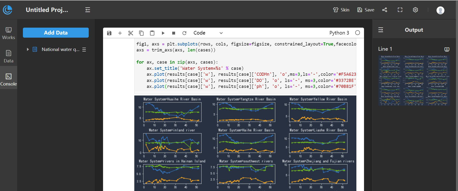
After successfully connecting to the DataScience service, a new blank Notebook will be created by default. On this Notebook page, you can write and run Python code. It also supports dragging and dropping local .py format files into the IN input box to run directly. In addition, the data in DataInsights is supported as the data source of Notebook; operation: From the data expanded on the left, click and drag a data field in the list to the variable row on the right that needs to be assigned a valu
After writing the code, click on ![]() on the toolbar to run. Analysis results (such as pictures, charts, texts, iFrames, etc.) will be synchronously output to the "Output" panel on the right; each result in the "Output" panel can be added to the DataInsights workbench; operation: Click on the right Create Card icon
on the toolbar to run. Analysis results (such as pictures, charts, texts, iFrames, etc.) will be synchronously output to the "Output" panel on the right; each result in the "Output" panel can be added to the DataInsights workbench; operation: Click on the right Create Card icon ![]() to add results into your workbench with one click.
to add results into your workbench with one click.
The following example shows analysis results of the PH value, DO (dissolved oxygen degree), and CODMIN (permanganate index) of each watershed based on the national watershed data in a certain year. In the figure, green represents PH value, orange represents CODMIN (permanganate index), and blue represents DO (dissolved oxygen).
Note 1: Currently Notebook files are not supported to be uploaded; the written code cannot be saved. Refreshing the page will clear the code, and you need to reconnect to the service;
Note 2: If the error "ModuleNotFoundError: No module named xx" is reported when running code, that means you need to install the corresponding missing modules on the DataScience server you use.