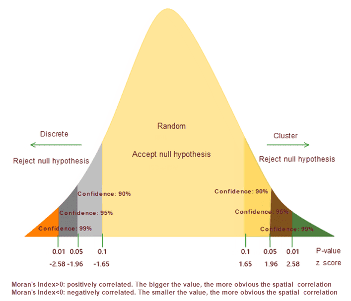
According to the specified features and related attributes, the mode expressed by the Global Moran’s I is cluster mode, discrete mode or random mode.
How Spatial Autocorrelation works
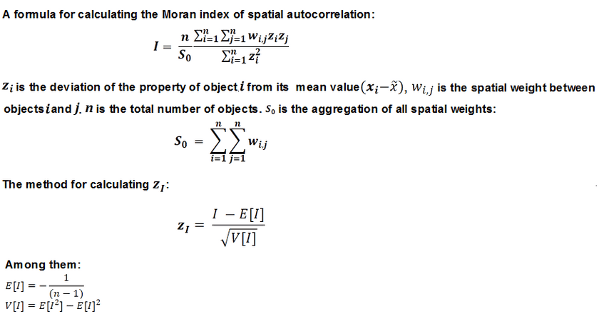
The statistical values of spatial autocorrelation can be calculated according to the following formula:
The math behind the Global Moran’s I statistic is shown above. The tool computes the mean and variance for the attribute being evaluated. Then, for each feature value, it subtracts the mean, creating a deviation from the mean. Deviation values for all neighboring features (features within the specified distance band, for example) are multiplied together to create a cross-product. Notice that the numerator for the Global Moran’s I statistic includes these summed cross-products.
After the Spatial Autocorrelation (Global Moran’s I) tool computes the Index value, it computes the Expected Index value. The Expected and Observed Index values are then compared. Given the number of features in the dataset and the variance for the data values overall, the tool computes a z-score and p-value indicating whether this difference is statistically significant or not. Index values cannot be interpreted directly; they can only be interpreted within the context of the null hypothesis.
Applications
- Help identify an appropriate neighborhood distance for a variety of spatial analysis methods by finding the distance where spatial autocorrelation is strongest.
- Measure broad trends in ethnic or racial segregation over time?is segregation increasing or decreasing?
- Summarize the diffusion of an idea, disease, or trend over space and time?is the idea, disease, or trend remaining isolated and concentrated, or spreading and becoming more diffuse?
Function Entrances
- Spatial Analysis > Spatial Statistical Analysis > Analyzing Mode > Spatial Autocorrelation. (iDesktop)
- Spatial Statistical Analysis > Analyzing Mode > Spatial Autocorrelation. (iDesktopX)
- Toolbox > Spatial Statistical Analysis > Analyzing Mode > Spatial Autocorrelation. (iDesktopX)
Main Parameters
- Source Dataset : Set up the vector data sets to be analyzed, supports points, lines, and regions three types of datasets. It is suggested that the number of objects in the source data is greater than or equal to 30 to ensure the reliability of the results.
- Assessment Field : Specify a numerical field for the analysis.
-
Concept Model : Your choice for the Conceptualized Model should reflect inherent relationships among the features you are analyzing. The more realistically you can model how features interact with each other in space, the more accurate your results will be.
- Fixed Distance:applicable to point and region with large changes in region size.
- Region Adjacent (Common Edges or Intersect): applicable to the data of adjacent side and intersection.
- Region Adjacent (Adjacency Point, Common Edges or Intersect): applicable to the region data with adjacent points,adjacent sides and intersecting.
- Inverse Distance: all features are regarded as adjacent features of all other features. All features affect the target features, but as distance increases, the effect is smaller, and the weight between the elements is one over the distance, which is applicable to continuous data.
- Inverse Distance Square: similar to the “Inverse Distance Model”, with the increase of distance, the influence decreases faster, and the weight between the features is one over the square of the distance.
- k-Nearest: The K features closest to the target features are contained in the calculation of the target features (the weight is 1), and the remaining features will be excluded from the target feature calculation (the weight is 0). This option is very effective if you want to ensure that you have a minimum number of contiguous features for analysis. This approach works well when the distribution of data changes in the study area so that some features are removed from all other features. When the proportion of fixed analysis is not as important as the number of fixed adjacent objects, k-nearest neighbor method is suitable.
- Spatial Weight Matrix File: space weight matrix file is required. The spatial weight is a number that reflects the distance, time, or other cost of each feature and any other feature in the dataset. If you want to model the accessibility of city services, for example, to look for areas where urban crime is concentrated, it is a good idea to use the network to model spatial relationships. Before analyzing, create a spatial weight matrix file (.swmb) using the generated network space weight tool, and then specify the full path of the SWM file created.
- Undifferentiated Regional: The model is a combination of “Inverse Distance Model” and “Fixed Distance Model”. Each feature is regarded as an adjacent feature of other features. This option is not suitable for large datasets. The features within the specified fixed distance range have equal weights (weights 1);In addition to the specified distance of fixed distance, the effect will be smaller as distance increases.
- Break Distance Tolerance : “-1” means to calculate and apply the default distance, which is to ensure that each element has at least one adjacent feature;” 0 “means that no distance is applied, and each feature is an adjacent feature. Non-zero positive values are adjacent features when the distance between the features is smaller than this value.
- Inverse Distance Power Exponent :The higher the exponent, the higher the power value, the smaller the exponential effect.
- Number of Adjacent Features :Set a positive integer, indicating that the nearest K features around the target features are adjacent features.
- Measure Distance Method : Currently, only Euclidean distance calculation and Manhattanis distance calculation are supported, for more specific instructions about the two calculations, please refer to Basic Vocabulary of Spatial Statistical Analysis.
- Spatial Weights Matrix Standardization :When the distribution of elements is likely to deviate due to sampling design or the aggregation scheme imposed, the use of the Spatial Weights Matrix Standardization is recommended. After selecting it, each weight is divided by the sum of the rows (the sum of the weights of all adjacent features). The normalized weights are usually used in combination with the fixed distance adjacent features and are almost always used for the adjacent features of the adjacent side. This can reduce the deviation caused by the different number of adjacent features. Spatial Weights Matrix Standardization takes ownership weights, making them between 0 and 1, creating relative (rather than absolute) weight solutions. Whenever you want to handle the region features that represent administrative boundaries, you might want to choose the “Spatial Weights Matrix Standardization” option.
Results Description
The output is a CAD dataset and displays on the map window.
The Spatial Autocorrelation returns five values: the Moran’s I Index, Expected Index, Variance, z-score, and p-value. Using z-score or p-value indicates statistical significance, you can refuse to null hypothesis, if Moran ‘s index value is positive, I have said this data with spatial correlation, the analysis of the dataset is used to value is proportional to the spatial concentration; If Moran’s I index is negative then indicates the discrete trend.
Instance
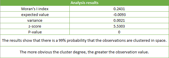
The following figure is the result of spatial autocorrelation analysis of the ratio and the number of cases of viral hepatitis in a county in a year. The Concept Model is set to Inverse Distance , the Measure Distance Method is set to Euclidean Distance , check the Spatial Weight Matrix Standardization checkbox, and other parameters are set to default values.
The results show that the P value is less than 0.01, Z score is greater than 2.58, and distribution is clustering distribution with 99% confidence. Moran’s Index greater than 0 (positively correlated) shows that the number of incidents in that year is highly clustered.


