An iteration loop refers to automatically repeating a process. It is mainly used in situations where repetitive tasks need to be performed automatically. Compared to manually executing repetitive tasks, iteration loops can greatly save the time and effort required to perform tasks. Iteration loops are divided into two modes: pairing loop and nested loop. The default mode is pairing loop.
- Pairing loop: It means performing one-to-one matching for each data in the collection data in order. Note that when the numbers of elements are m and n respectively, the number of executions is the minimum of m and n. That is, when m > n, the loop will only execute n times.
- Nested loop: It means performing cross-loop matching for each data in the collection data.
Feature Description
1. Connect the collection dataset to a single-value input.
2. Right-click the tool node - Iteration Mode - pairing loop/nested loop.
3. Note that the iteration loop is only meaningful when used in multiple loops.
4. The iteration loop is only meaningful when used with a single-value input; otherwise, the correct iteration result cannot be obtained.
Use Case 1: Batch Processing of Iterate Datasets
When the number of datasets in the data source is very large, iterate datasets can be used for batch processing of data. When performing iteration loops on iterate datasets, the iteration mode can be selected according to the actual situation to achieve iterative batch processing.
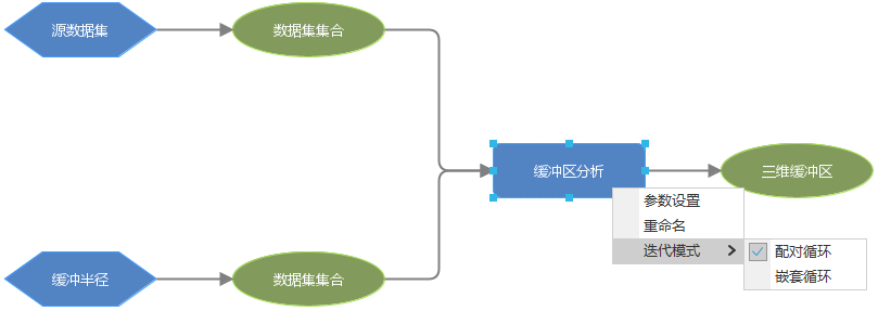
In the model below, buffer analysis needs to be performed on iterate datasets. When two iterate datasets are connected to the buffer analysis tool node, the iteration mode can be selected, and then the model can perform pairing loop or nested loop on the two iterate datasets during runtime.
Use Case 2: Batch Processing of Collection Variables
Variables support creating collection data and can batch set multiple data. At the same time, collection variables support selecting data across data sources. By using iteration loops, batch processing can be achieved. For example, performing buffer analysis on three data in a certain area, the specific steps are as follows:
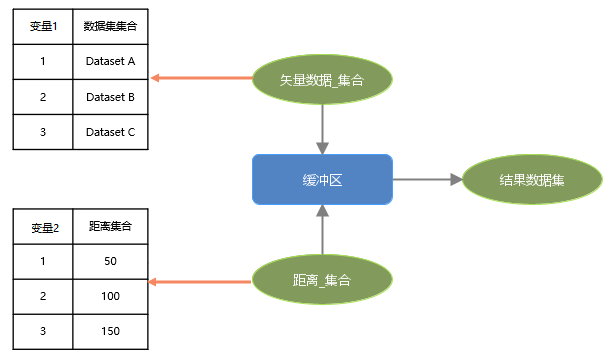
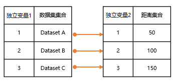
Create a collection variable: Click the "GPA" tab, select the "Variable" group, and the drop-down menu will display a list of all data types that can be used in the model. Double-click the variable of vector dataset type, check the collection option, then you can add three vector datasets via the "Add" button in the properties panel. Next, create an integer variable and add buffer distances, setting three distances: 50, 100, and 150. Construct the following model on the canvas:
Select the Buffer tool node, and you can choose pairing or nested loop via the context menu. The differences between the two loop modes are as follows:
Pairing loop. As shown in the figure below, according to the data correspondence, Dataset A corresponds to distance 50; Dataset B corresponds to distance 100; Dataset C corresponds to distance 150, and buffer analysis is performed separately, ultimately obtaining three results.
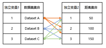
Nested loop. As shown in the figure below, Dataset A is analyzed three times according to distances 50, 100, and 150; similarly, Dataset B and Dataset C are also analyzed according to the three distances respectively, ultimately obtaining nine results.
Use Case 3: Batch Processing of Datasets
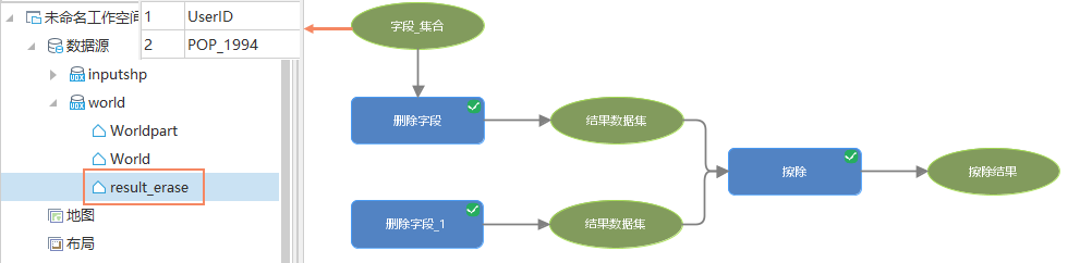
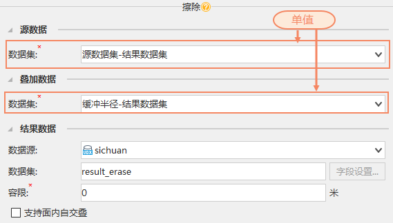
When batch processing source data, sometimes only one result dataset needs to be output. For example, mass delete the UserID and POP_1994 fields in the World dataset, and then erase the Worldpart dataset from the World data.
According to the principle of nested loop, since two values are filled in the Field_Collection, the Erase will be executed twice, generating two result datasets: result_erase and result_erase_1. These two datasets are the same, so by default, the calculate result is intelligently deduplicated, ultimately obtaining one result dataset result_erase, avoiding resource waste.