Instructions for use

In the case of biased samples, the existing data or covariates are used to calculate the correlation coefficient between each two samples, that is, the sample and the population, the sample mean and the population mean (the ratio of the estimated target), so as to realize the unbiased estimation of the biased sample to the population mean.

(Biased sample: In statistical research, the data used to estimate the parameter under study depends on a sample drawn from the population. If the samples are random, that is, the samples are obtained in a way similar to "drawing lots", the parameters estimated from these sample data can accurately reflect the relevant characteristics of the population. The theory is that the estimated parameters are unbiased; but if the samples are not random, then the parameters estimated from these samples do not accurately reflect the distribution of the population properties under study. However, most of the sampling is not random, but only within the scope and rules chosen by the researchers, which may lead to sampling bias.

When there is sufficient Historical Data or prior information to measure the ratio of each sample point to the target population (total or mean), and the covariance between two samples in the population can be calculated, the model can significantly improve the estimation accuracy. The B-Shade model makes full use of the horizontal correlation of geographic space and the vertical correlation between the sample and the regional population, and is widely used in the Statistical Inference with biased samples. Even if the sample is biased, the B-shade model can also be used to obtain the optimal unbiased estimation of the regional population.

Function entrance

• Spatial Statistical Analysis tab-> Spatial Sampling and Statistical Inference-> Bshade Sampling. (iDesktopX)
• Toolbox-> Spatial Statistical Analysis-> Spatial Sampling and Statistical Inference-> Bshade Sampling. (iDesktopX)

Parameter Description

• Historical Data: The specified Historical Data set and its Datasource. The following case shows the morbidity data of 19 hospitals last year.
• Parameter Settings：

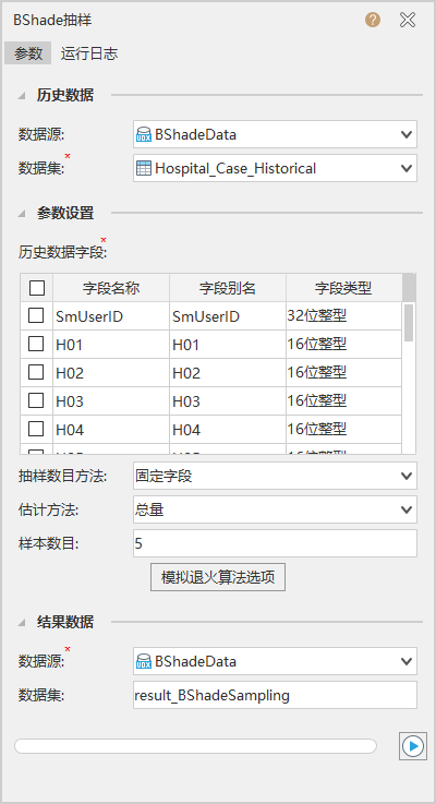
Historical Data Field: Check the specified Historical Data set data field. In the following case, 19 fields are checked for recording the data of 19 hospitals in the last year.

Sample Number Method: Select Fixed Field or Extent Field.

• Fixed field: that is, the fixed number of samples with the smallest estimated difference is obtained by sampling. In the following cases, the Number of Samples is set to 5, which means that the 5 hospitals with the smallest estimated difference are selected as the best sampling selection.
• Extent Field: All sample selections and corresponding estimated variances will be generated according to the set upper limit, lower limit, and step size of the number of samples. The best solution can be chosen based on the smallest possible number of samples (reduced cost) and the smallest possible estimation variance (higher accuracy).

Estimation method: BShade estimation method. The aggregate method is based on the ratio of the sample to the population, and the mean method is based on the ratio of the sample mean to the population mean.

Number of samples: The number of samples taken.

Simulated Annealing Algorithm Options: Simulated annealing algorithm is a general optimization algorithm, which is based on the similarity between the annealing process of solid matter in physics and the general combinatorial optimization problem. Starting from a higher initial temperature, with the continuous decline of the temperature parameter, the global optimal solution of the objective function is randomly searched in the solution space combined with the probability jump characteristic, that is, the local optimal solution can jump out of the local optimal solution in probability and finally the global optimal solution is obtained. Parameters include start temperature, minimum temperature, minimum energy, annealing rate, maximum number of rejections, maximum number of attempts, maximum number of successes, and maximum number of combinations. Has a default value.

• Result Data: Set Result Dataset and its Datasource.
• Click the Execute button to execute the prepared analysis function. After the execution completed, the Output Window will prompt whether the Result succeeds or fails.

Application case

A region needs to get the daily incidence of a disease in a certain month of this year. Because there are many hospitals, the data collection of all hospitals is time-consuming. Now we need to sample the designated hospital as a sample, and then get the prediction results. Before the prediction, the morbidity data of last year of 19 designated hospital in the region have been collected as a reference. Using the Bshade Sampling function, 5 hospitals with the smallest estimated variance can be extracted as samples, and the incidence data of these 5 hospitals this year can be used for prediction and analysis.

• Case Data: Click here to download < a class = "contentpage hyperlink" href = "./data/BShadeData. Zip" "=" "> Bshade Sampling and Predicted Case Data , download and unzip. The data involved in the analysis are: Hospital _ Case _ Historical, which is the historical incidence data of all hospitals in the region.
• Parameter Settings: After downloading the above case data, open the BShadeData. Udbx on the desktop, perform Parameter Settings as shown in the following figure, and execute Bshade Sampling analysis. In this case, the method of Extent Field is used for sampling, and multiple groups of sampling results are obtained according to the set upper limit, lower limit and step length of the sampling number.



• Results: After the analysis by the Extent Field method of Bshade Sampling, multiple groups of samples can be obtained. Finally, we select the last group as the sample hospital, and sort out the recent incidence data of these five hospitals for the later Bshade Estimation analysis. Result Data is shown as follows: