


Application provides histogram function, which is convenient for users to view the distribution of sampling points. On the Spatial Analysis tab, click the Histogram button in the Raster Analysis group to view a histogram of the sampled data.
Histogram, also known as frequency distribution histogram, provides the frequency distribution map of a field grouping of sampling point data and summarizes Statistical Data. The area of each bar represents the relative frequency within a particular partition or group. The number of equal width classes used by default in the histogram. The following figure shows the frequency distribution of one field of a Dataset (15 groups):
 |
| Figure: Sample Point Histogram |
By using the histogram, the shape of the sample distribution can be examined. By observing the summarized Statistic Infomation, we can understand the location distribution, shape, dispersion and so on of the data. For example, by comparing the Statistics Result of the mean and median, it is easy to locate the center of the sample distribution. When the mean and median are very close, the data can be considered to be normally distributed.
 Histogram dialog description
The upper chart area of the dialog box is mainly used to display the histogram and Statistic Infomation, and the lower part is used to set the statistical data and parameters of the histogram.
Chart Area
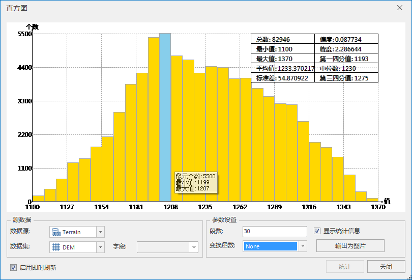
The horizontal axis (X axis) of the histogram represents the value of each sample point, and the vertical axis (Y axis) represents the number of sample points. The Statistics Result of all sample points is displayed in the upper right corner of the histogram, including the total number of sample points, the minimum value, the maximum value, the average value, the standard deviation, the kurtosis, the first four scores, the median, and the third four scores.
Source Data
Datasource: All the Datasources in Current Workspace are listed. Select the Datasource where the Point Dataset to be analyzed is located.
Dataset: All Point Datasets in Source Datasource are listed. Select a Point Dataset as the analysis Dataset.
Parameter Settings
Number of segments: Enter a positive integer as the number of Statistic Analysis segments, i.e., the number of histograms.
Transformation function: It is a function that transforms the field value. The system provides three transformation functions: NONE (no function, i.e. no transformation), LOG (logarithmic function) and ARCSIN (arcsine function). When the transformation function interpolates the sample data, some interpolation methods (such as Ordinary Kriging, Simple Kriging and Universal Kriging) assume that the data obey the normal distribution. If the sample data do not obey the normal distribution, it is necessary to transform the data so that the data obey the normal distribution. The three transform processing functions are described as follows:
- None: No function, that is, no transformation processing is performed, and Source Data is used for interpolation.
- Log: Logarithmic function, that is, logarithmic transformation of Source Data with natural logarithm as base. Logarithmic transformation is applicable to the sample data with a positively skewed distribution, that is, the peak is to the left, that is, the median is greater than median. The domain of the log function is a real number greater than 0, so make sure this condition is met when making changes to the log function.
- Arcsin: Arcsine function, that is, arcsine transform of Source Data. The arcsine function works well for data that is proportional or distributed in percentages. The domain of this function is -1,1, so be aware of the value range of the Statistic Field when performing the arcsine transformation.
Show Statistics: Select the check box to display the Statistic Infomation of the histogram in the upper right corner of the dialog box. When the check box is not selected, Show statistics is not displayed.
Statistic Infomation
- Total: The total number of Point Dataset objects.
- Min/Max/Avg/Std: Min/Max/Avg/Std of the Statistics Result in the histogram.
- Skewness: It is used to describe the symmetry of distribution. If the distribution is symmetric, the value is 0; if the distribution is skewed to the left, the value is positive and the mean is greater than median; if the distribution is skewed to the right, the value is negative and the mean is less than median.
- Kurtosis: An indicator used to describe the likelihood of outliers in a distribution. The value is 3 for a normal distribution, greater than 3 for a peaked distribution, and less than 3 for a flattened distribution.
- The first four scores/the third four scores: 0.25 times and 0.75 times of the cumulative proportion respectively. That is, All Data is sorted in ascending order, with the first quartile representing the value at 1/4 of the sorted data and the third quartile representing the value at 3/4 of the sorted data.
- Median: equivalent to 0.5 times the cumulative proportion respectively. That is, All Data is sorted in increasing order, and the median represents the value at 1/2 in the sorted data. If the amount of data is even, there are two medians, and the first median is taken here as the value.
Export as Image: Export the histogram as image. The supported image formats include: BMP, EMF, EPS, JPG, PNG, TIF, etc.
 Remark
When the mouse slides over or selects a column bar in the histogram, the information of the column bar will be displayed in real time, including the objects contained in the data and the minimum/maximum values.
- Object Count: the number of corresponding point objects of the selected histogram.
- Min/Max: Select the minimum/maximum value of the histogram Statistics Result.