


Distance Raster Analysis is to analyze the Spatial Distance of each grid from its neighboring pixels (sources), so as to reflect the spatial relationship between each pixel and its neighboring pixels. It not only considers the grid surface distance, but also considers the influence of various consumption factors such as cost. Through distance analysis, a lot of useful information can be obtained to guide people to manage and plan resources, such as the distance between the earthquake emergency rescue area and the nearest hospital, the service area evaluation of supermarket chains, etc.
Distance Raster Analysis mainly includes three aspects:
- One is Generate Distance Raster, which calculates the distance between each cell and the nearest source (the object of interest), including Straight-line Distance, Cost Distance and Surface Distance, and generates the corresponding direction grid and distribution grid;
- Condly, according to the direction grid and the distribution grid, the Shortest Path from the target to the source is analyzed and obtained;
- The third is to calculate the Shortest Path between two points (source point and target point), including the minimum cost path and the shortest surface distance path.
Basic concepts
Let'sstart with the basic concepts related to Raster Analysis.
Source: Objects or features of interest, such as schools, roads, or fire hydrants.
Source Dataset: Dataset containing the source, which can be a 2D point, line, Region Dataset, or Raster Dataset. For Raster Dataset, requires cells other than identity source to have no value.
Distance: includes Straight-line Distance, Cost Distance, and Surface Distance, as described below:
- The Straight-line Distance is the Euclidean distance, which is the Straight-line distance from each cell to the nearest source.
- The cost distance is the cost value required to actually reach the nearest source obtained according to the weighting of one or several attribute factors of the cell;
- The surface distance is the actual surface distance from the cell to the nearest source, calculated from the surface grid.
Straight-line Distance can be seen as the cost of length, which is the simplest kind of cost. On the other hand, the actual land cover types are diverse, and it is almost impossible to reach the source through the straight-line distance, and it is necessary to make a detour to avoid obstacles such as rivers, mountains, and so on. Therefore, it can be said that the cost distance is the expansion and extension
of the straight-line distance.Cost grid: The cost grid is required for the Generate Cost Distance Raster and for calculating the minimum cost path. The cost grid is used to determine the cost required to pass through each cell. The value of the cell represents the cost of one unit passing through the cell and cannot be negative. For example, if the grid value of a cost grid representing the forward resistance of a vehicle in different ground environments represents the resistance value for each kilometer of advance when passing through the cell, then the total cost of passing through the cell is the unit cost value (i.e., the grid value) multiplied by the size of the cell. The units that cost the grid can be any unit type, such as length, time, money, etc., or unitless, such as regraded slope, aspect, Land Use type, etc.
3.Calculate the Shortest Path between two points
 Generate Distance Raster
The Generate Distance Raster function is used to calculate the distance between each pixel of Raster Data and the source data. The results obtained can be used to solve three problems:
- The distance from each pixel
- in Raster Data to the nearest source data, such as the distance to the nearest school. The direction of each pixel
- in Raster Data to the nearest source data, such as the direction to the nearest school. Pixels to be assigned to the source data
- according to the spatial distribution of the resource, such as the nearest several school locations.
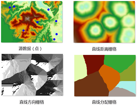
Generate Distance Raster results in three types of Datasets, namely the Distance Raster, the Direction Grid, and the Distribution Grid. As shown in the following figure, the three grids are shown separately.
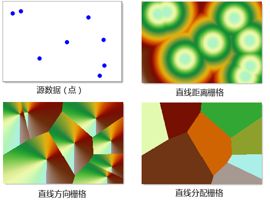 |
Distance Raster
Distance Raster includes Line Distance Raster and cost Distance Raster.
- Line Distance Raster The value of the
Line Distance Raster represents the Euclidian distance (or Straight-line Distance) of the cell to the nearest source. Straight-line Distance can actually be regarded as the simplest kind of cost with length as the cost. The Line Distance Raster does not consider cost, that is, the route is considered to be free of obstacles or equivalent cost. The source data for generating the Line Distance Raster can be either Vector Data (point, line, surface) or Raster Data. The results of the analysis include Line Distance RasterDataset, line direction Raster Dataset, and line assignment Raster Dataset.
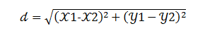
Line Distance Raster is the result of calculating the Euclidean distance of each cell from the nearest source. Assuming that the coordinates of point A are (x1, Y1) and the coordinates of point B are (x2, Y2), the Euclidean distance between the two points AB is:
- Cost distance The value of the
Cost Distance Raster represents the value of the cost to the nearest source for that cell (which can be various types of cost factors, or a weighting of each cost factor of interest). For example, the journey over a mountain is less expensive, but if you consider the time cost, it may be more expensive than time cost around it. On the other hand, the actual land cover types are diverse, and it is often impossible to reach the source through the Straight-line Distance, and it is necessary to make a detour to avoid obstacles such as rivers, mountains, etc., so it can be said that the distance is consumed to expand and extend the Straight-line Distance. Because Distance Raster records the distance from each cell to the nearest source (resource point), through Distance Raster, we can take "the distance that the user expects to be less than nearest resource point" as the location condition, thus serving the location analysis.
Directional Grid
The orientation grid represents the azimuthal orientation between each grid pixel and the nearest source. It can also be divided into linear directional grid and linear directional grid. The value of the straight direction grid indicates the azimuth of the cell to the nearest source in degrees. Rotate in a clockwise direction from 0 to 360 degrees with the direction of due north as 0 degrees. For example, if the nearest source is due east of the cell, the value of the cell is 90 degrees.
The value of thecost direction grid expresses the direction of travel of the least-cost path from the cell to the nearest source. As shown in the figure below, in the Raster Data shown in Figure 1, the minimum cost route for each cell to reach the source (identified by a small red flag in the figure) is identified by an arrow. Since the value of the direction is specified as shown in Figure 2, the value of the direction of each cell in Figure 1 is shown in Figure 3. Figure 3 shows the cost direction grid of the Raster Data of Figure 1. The value in the consumption direction Raster Dataset is 0 for the cell where the source is located. Of course, not all cells in the Direction Dataset with a grid value of 0 are sources. For example, a cell with no value in the input Raster Dataset also has a value of 0 in the output Cost Direction Dataset.
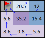 | 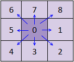 | 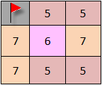 |
| Figure 1 | Figure 2 | Figure 3 |
Assign Grid
Gridallocation is to allocate spatial resources (grid pixels) to different source objects, for example, it can represent the service areas of multiple post offices, which is convenient for customers to select the nearest post office for service.
The allocation grid includes a linear allocation grid and a cost allocation grid. The allocation grid is also called the service area grid, and its grid value is the value of the nearest source, so you can know which is the nearest source of each cell from the allocation grid. When calculating the straight-line distance, the nearest source is determined by the straight-line distance between the cell and the source; when calculating the cost distance, the nearest source is determined by the cost distance between the cell and the source.
In thefigure below, the source data is Point Dataset, the DEM data is Cost Data, and the Raster Data result is obtained by Generate Cost Distance Raster.
 |
Compute Shortest Path
The Shortest Path Analysis is based on the target point data and the Distance Raster and orientation grid generated by the Generate Distance Raster "feature. Calculate the Shortest Path of the target to the nearest source, such as the Shortest Path from a suburban point to the nearest shopping mall (Target Dataset).
For example, analyze how to get to the nearest shopping mall (Point Dataset) from each residential area (Region Dataset). First, the shopping mall is used as the source, Generate Cost Distance Raster and consumption direction grid; Taking the residential area as the target area, the Shortest Path from each residential area (target) to the nearest shopping mall (source) can be obtained by Shortest Path Analysis based on the generated cost Distance Raster and cost direction grid.
There are three Path Types forCompute Shortest Path:
- Pixel Path: Each grid pixel generates a path, that is, the distance from each target pixel to the nearest source.
As shown in the figure below, the red point is used as the source, and the black frame polygon is used as the target. In this way, the grid Shortest Path Analysis is performed, and the Shortest Path represented by the blue cell is obtained.
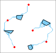
Figure: Pixel Path Analysis - Zonal Path: Each grid area generates a path. Here, the grid area refers to a continuous grid with equal grid values. The Zonal Path is the Shortest path from each target area to the nearest source.
As shown in the figure below, the red point is used as the source, and the black frame polygon is used as the target. In this way, the grid Shortest Path Analysis is performed to obtain the Shortest Path represented by the blue cell.
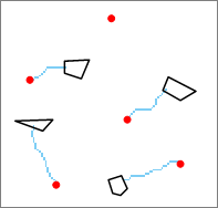
Figure: Zonal Path Analysis - Single Path: Only one path is generated for all pixels, which is the shortest path for the entire target Area Dataset.
As shown in the figure below, the red point is used as the source, and the black frame polygon is used as the target. In this way, the grid Shortest Path Analysis is performed, and the Shortest Path represented by the blue cell is obtained.
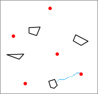
Figure: Single Path Analysis
Compute two-point Shortest Path
Calculate the Shortest Path between the source and destination points. Based on the specified surface grid or cost grid, you can calculate the shortest surface distance path, the minimum cost path, or the minimum cost path considering the surface distance between two points.
Cost distance
Computing the minimum cost path requires specifying the cost grid. The cost grid is used to determine the cost required to pass through each cell. The value of the cell represents the cost of one unit passing through the cell. For example, if the grid value of a cost grid representing the forward resistance of a vehicle in different ground environments represents the resistance value for each kilometer of advance when passing through the cell, then the total cost of passing through the cell is the unit cost value (i.e., the grid value) multiplied by the size of the cell. The units that cost the grid can be any unit type, such as length, time, money, etc., or unitless, such as regraded slope, aspect, Land Use type, etc. Usually, there may be many factors affecting the cost involved in an actual study. For example, when planning a new road, the factors affecting the cost may include the total length of construction, the Land Use type of the area it passes through, the slope, the distance from the population gathering area, etc. These factors need to be weighted to get a combined weight as Cost Data. In addition, it is important to note that the cost cannot be negative.