OLS (Ordinary Least Squares) is the simplest and most commonly used method. It can not only provide a global model for the variable or process you want to know and predict, but also create a regression equation to represent the process. Geographically Weighted Regression (GWR) is one of the spatial regression methods used in geography and other disciplines. It provides a local model for the variable or process to be predicted by fitting a regression equation to each element in the dataset.
 Instructions
Function entrances:
- Spatial Analysis tab > Spatial Statistical Analysis > Modeling Spatial Relationship > Ordinary Least Square.
- Toolbox > Spatial Statistical Analysis > Modeling Spatial Relationship > Ordinary Least Square.
Major Parameters
- Source Data: specify the vector dataset that you want to analyze. The supported datasets can be point, line, and region. Note: the dataset must have at least 3 objects.
- Explanatory Variable: The explanatory variable is the independent variable (X in the regression equation). You can check one or more numerical fields to model or predict the value of the dependent variable. Note: if all values of an explanatory fields are the same, the OLS regression equation has no solutions.
- Model Field: the dependent variable to be researched or predicted. The filed must be numerical. iDesktopX can build a regression model according to known observation values to get the predicted independent variable.
- Result Data: specify a datasurce to save the resulting data with the same type as the source data.
Output
The resulting prediction values, residuals, and standard residuals are recorded in attribute fields of the resulting dataset. While the distribution statistics, percentage, AICc, and coefficient are output in the output window.
1. Records in the resulting attribute table
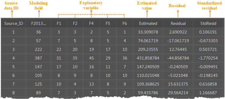
- Source_ID: SmID values of objects in the source dataset.
- Model Field and Explanatory Fields: retains original model field and explanatory fields.
- Estimated: fitted values obtained by an OLS analysis according to specified explanatory fields.
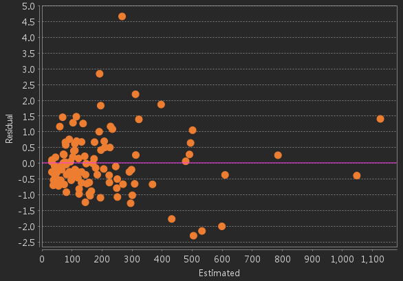
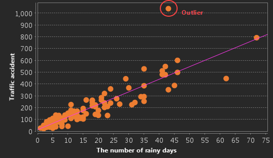
- Residual: The differences between estimated values and actual values. The mean of the standardized residual is 0, and the standard deviation is 1. You can use residuals to determine the fitting degree of the model. Small residuals indicate that the model fits well and can predict most of values, which means this regression equation is effective. You can perform spatial autocorrelation analysis on the residuals. If the clustering of either the high residuals or low residuals is statistically significant, your model must be missing a key variable. In this case, the OLS result is unreliable. The scatter plot in the figure below shows relationships between the model residuals and the predicted values. If you are modeling the traffic accident rate, the model can predict locations with a low traffic accident rate, but cannot predict the areas with high traffic accident rates.
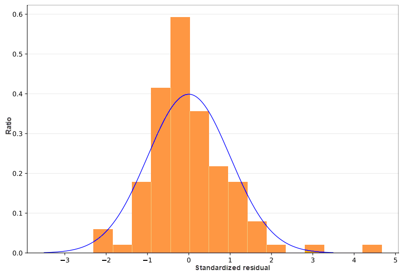
- StdResid Residual: The standard residual is the ratio of the residual to the standard error. It can be used to judge whether your data is abnormal. If the standard residuals present a normal distribution, the performance of the model is relatively excellent. But if there is a severe skew, the model is biased, which means the model misses a key variable. If your data ranges from -2 to 2, it has normality and homogeneity of variance. But if your data exceeds the range of (-2, 2), it is abnormal and has no homogeneity of variance and normality. The residuals in the figure below are non-normally distributed and have a certain offset.
You can make a residual range thematic map to check which areas have high or low residuals, analyze the clustering areas that have high and low predicted values, and learn which explanatory variables may miss from the distribution characteristics of residuals.
2. Table in the output window
- Coefficient: The coefficient reflects the strength and type of relationship between each explanatory variable and the dependent variable. The greater the absolute value of the coefficient, the greater the contribution of the variable to the model, and the closer the relationship. The coefficient reflects the expected amount of change in the dependent variable per unit change of the associated explanatory variable when all other explanatory variables remain unchanged. For example, keeping other explanatory variables constant, for every additional person in the census block, the burglary coefficient will increase by 0.005. At the same time, the coefficient also indicates the type of relationship between the explanatory variable and the dependent variable. A positive coefficient indicates a positive correlation. For example, the greater the population, the greater the number of burglaries. A negative coefficient indicates a negative correlation, such as the closer to the town centers, the fewer the number of burglaries.
- Coefficient Standard Deviation: the dispersion degree of different explanatory variables.
- Standard Error: these values are used for measuring the reliability of the estimated value of each coefficient. The smaller the value, the higher the reliability. While a big standard error means there is the multicollinearity problem.
- t-Statistic: It is used for estimating whether an explanatory variable is statistically significant. t-Statistic equals the standard error divided by the mean. In general, this value has the same meaning as P-value. Both of them are used for verifying the significance of models in null hypothesis testing. But sometimes P-value will have some problems, such as missing some information. When performing statistical verification, the larger the t statistic, the more significant data is.
- Probability: if the p-value is very small, the probability that the coefficient is 0 is very low.
- Robust Coefficient Standard Errors: checks whether the regression coefficient and result of the explanatory variables are robust by modifying variable values.
- Robust Coefficient: it is used for estimating whether the robust coefficient is statistically significant.
- Robust Coefficient Probability: if Koenker (Breusch-Pagan) is statistically significant, the method will use the robust coefficient probability to estimate the statistical significance of explanatory variables.
- Variance Inflation Factor (VIF): this value is used for verifying whether there are redundant explanatory variables (multicollinearity). In general, if the value of a variable is bigger than 7.5, the variable is redundant probably.
3. The resulting list in the output window
- AIC: it is a criterion for evaluating how well a model fits data.It can compare different possible models and determine which one is the best fit for the data.AIC encourages the fit of the data, but overfitting should be avoided as much as possible. Therefore, the smaller AIC value should be in consideration first is to find a model that can best interpret the data but contains the fewest independent variables.
- AICc(Akaike): When data increases, AICc is the measure of model performance as well. Considering the complexity of the model, a model with a lower AICc value can better fit the observed data. AICc is not an absolute measure of goodness of fit, but it helps compare models that use the same dependent variable and have different explanatory variables. If the difference of the AICc values between the two models is greater than 3, the model with the lower AICc value will be considered the better model.
- Coefficient Determination (R2): The coefficient of determination is a statistical measurement. Its value varies between 0.0 and 1.0. The larger the value, the better the model. R2 is the proportion of the variance in the dependent variable covered by the regression model. The denominator calculated by R2 is the sum of the squares of the dependent variable values. Adding an explanatory variable will not change the denominator but will change the numerator, which may improve the model fit.
- Adjusted Coefficient Determination: The calculation of the adjusted coefficient of determination will normalize the numerator and denominator according to their degrees of freedom. Since the adjusted R2 value is usually less than the R2 value, the normalization can compensate the number of variables. However, the interpretation of this value can't be used as a proportion of the explained variance. The effective value of the degrees of freedom is a function of bandwidth. Hence, AICc is the preferred way to compare models.
The two coefficients range from 0 to 1 and can be converted into percentages, referring to the interpretative ability of the independent variable to the dependent variables. For example, if the value is 0.8, the regression equation can explain 80% of the change in the dependent variable. The higher the square coefficient, the higher their coincidence degree. The adjusted R-square coefficient is usually slightly lower than the multiple R-square coefficients. Since the technology of this coefficient has a stronger relationship with the data situation, the performance evaluation of the model is more accurate.
- Residual Variance: the effective degree of freedom of the residual sum of squares divided by the residual. The smaller the statistical value, the better the model fitting effect.
- Koenker (Breusch-Pagan) Statistic degrees of freedom:: The degree of freedom is related to the number of explanatory variables. The more explanatory variables, the greater the degree of freedom.
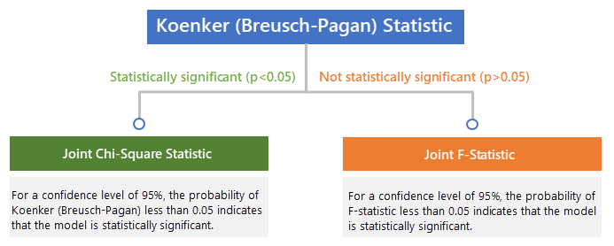
- Probability of Koenker (Breusch-Pagan) Statistic:: It is used for testing whether the Koenker (Breusch-Pagan) is statistically significant. For a confidence level of 95%, the probability of Koenker (Breusch-Pagan) less than 0.05 indicates that the model is statistically significant.
- Koenker (Breusch-Pagan) Statistic:: Koenker's standardized Breusch-Pagan statistics can assess the steady state of the model and determine whether the explanatory variables of the model have consistent relationships with the dependent variables in both geographic space and data space. For a confidence level of 95%, the probability of the Koenker (Breusch-Pagan) statistic is less than 0.05, indicating that the model has statistically significant heteroscedasticity or non-steady state. When the test result is statistically significant, you need to refer to the robustness coefficient standard deviation and probability to evaluate the effect of each explanatory variable.
- Joint Chi-Square Statistic degrees of freedom: The degree of freedom is related to the number of explanatory variables. The more explanatory variables, the greater the degree of freedom. In the chi-square distribution, the greater the degree of freedom, the closer the chi-square distribution is to the normal distribution.
- Probability of Joint Chi-Square Statistic: It is used for testing whether the Koenker (Breusch-Pagan) is statistically significant. For a confidence level of 95%, the probability of Koenker (Breusch-Pagan) less than 0.05 indicates that the model is statistically significant.
- Joint Chi-Square Statistic: It is used for testing the statistical significance of the entire model. Only when the Koenker (Breusch-Pagan) statistic is statistically significant, the joint F statistic is credible. The null hypothesis is that the explanatory variables in the model do not work. For a confidence level of 95%, the probability of the joint F statistic less than 0.05 indicates that the model is statistically significant.
- Joint F-Statistic degrees of freedom: The degree of freedom is related to the number of explanatory variables. The more explanatory variables, the greater the degree of freedom.
- Probability of Joint F-Statistic: It is used for testing whether the F-statistic is statistically significant. For a confidence level of 95%, the probability of F-statistic less than 0.05 indicates that the model is statistically significant.
- Joint F-Statistic: It is used for testing the statistical significance of the entire model. Only when the Koenker (Breusch-Pagan) statistic is statistically significant, the joint F statistic is credible. The null hypothesis is that the explanatory variables in the model do not work. For a confidence level of 95%, the probability of the joint F statistic less than 0.05 indicates that the model is statistically significant.
- Jarque-Bera Statistic degrees of freedom: The degree of freedom is related to the number of explanatory variables. The more explanatory variables, the greater the degree of freedom.
- Probability of Jarque-Bera Statistics: It is used for testing whether the Jarque-Bera is statistically significant. For a confidence level of 95%, the probability of the Jarque-Bera statistic less than 0.05 indicates that the model is statistically significant.
- Jarque-Bera Statistic: The Jarque-Bera statistic can evaluate the deviation of a model. It can be used to indicate whether the residual (the result of the dependent variable value minus predicted value) is normally distributed. The null hypothesis of this test is that the residual is normally distributed. If the p-value is small (for example, for a 95% confidence level, the value is less than 0.05), the regression will not be normally distributed, indicating that your model is biased. If the residual still has a statistically significant spatial autocorrelation, the deviation may be produced because of missing a key variable. Therefore, the result of the OLS model is unreliable.
Model Determination
After selecting the dependent variable and candidate explanatory variables, and doing OLS regression analysis, in order to find out whether a useful and stable model is found, the following diagnosis is required for the output test parameters.
- Which explanatory variables are statistical significant
- Coefficient: The larger the absolute value, the greater the contribution of the variable in the model. The closer to zero, the smaller the role of the relevant explanatory variable
- Probability: If the value is less than 0.05, it means that the relevant explanatory variable is very important to the model, and its coefficient is statistically significant with 95% confidence.
- Robust probability: If the probability of the Koenker (Breusch-Pagan) statistic is less than 0.05 and the robust probability is less than 0.05, the explanatory variable is significant.
- Relationship between dependent variable and explanatory variable
A positive explanatory variable coefficient indicates a positive correlation, and a negative value indicates a negative correlation. When creating the candidate explanatory variable list, each variable will have the correlation (positive or negative) expected by the user. In the analysis result, if the relationship between an explanatory variable and the dependent variable doesn't fit the theory, while other test parameters are normal, the dependent variable may be related to some new reasons, which will help improve the accuracy of the model. For example, the analysis results indicate that there is a positive relationship between the frequency of forest fires and rainfall. Lightning is likely the main cause of forest fires in the studied area.
- Whether the explanatory variable is redundant
When performing an analysis, to construct a model of different factors, we will select many explanatory variables. Therefore it is necessary to know whether there are redundant variables. The expansion factor (VIF) is a measure of the redundancy of variables. Based on the experience, a VIF value exceeding 7.5 may be a redundant variable. If there are redundant variables, please remove them and re-execute the OLS analysis. If the model is used for prediction and the results have a good fit, it is not necessary to deal with the redundant variables.
- Whether the model is biased
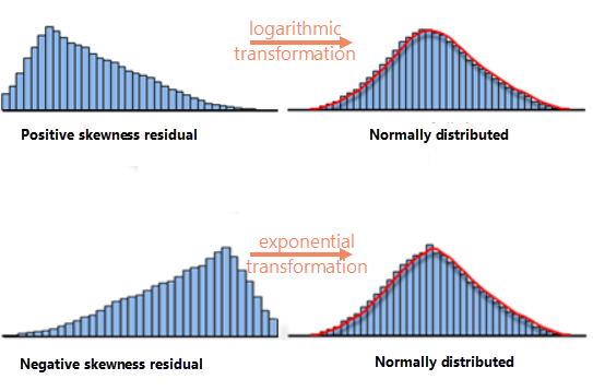
Model residuals can be used to judge whether the model has deviation. You can create a histogram for the model residuals field. If the model residuals are normally distributed, the model is accurate and unbiased; if the model residuals are not normally distributed, the model has deviation. If the model is biased, you can create a scatter plot for all the explanatory variables of the model to see if it is a non-linear relationship or outliers and you can correct it in the following ways:
- Non-linear relationship: This is a common cause of model deviation. Variable transformation can be used to make a linear relationship more obvious. Common transformations include logarithmic transformation and exponential transformation. The transformation method is selected by the distribution of the explanatory variable histogram, as shown in the following figure:
- Outliers: Check whether there are outliers in the scatter chart, and then analyze whether the outliers affect the model. Run OLS with and without outliers respectively to compare the degree to which the outliers change the model performance, and whether removing the outliers will correct model deviations. If the outliers are incorrect data, they can be deleted.
- Have all the key explanatory variables found
The statistically significant spatial autocorrelation phenomenon in the model residuals is evidence that you have lost one or more key explanatory variables. In regression analysis, the problems with spatial autocorrelation residuals usually exist together with the phenomenon of clustering: high predicted values are clustered together, and low predicted values are clustered together. Spatial autocorrelation analysis can be performed on the residual field. If the resulting P<0.05, the model has lost key explanatory variables.
- Model performance evaluation
After satisfying the above 5 conditions, the advantages and disadvantages of the model can be evaluated by correcting the R2 value. The R2 value ranges from 0 to 1, expressed as a percentage. Suppose you are modeling traffic accident rates and find a model that passes all five previous checks, with a corrected R2 value of 0.7. In this way, you can understand that the explanatory variable in the model indicates that the traffic accident rate is 70%, and it can also be understood that the model explains 70% of the change in the dependent variable of the traffic accident rate). Different fields have different requirements for the value of R2. In some scientific fields, being able to explain 25% of complex phenomena is enough to be exciting; in some fields, the R2 value may need to be close to 80% to be satisfactory.
The AICc value is also often used to judge models. The smaller the AICc value, the more suitable the observed data.
 Related Topics